python-ggseg

Python module for ggseg-like visualizations.

Dependencies

Requires matplotlib>=3.4, numpy>=1.21, and scikit-image>=0.19 (the last is used to resample 2D arrays when rendering them inside region outlines — see "Plotting arrays inside regions" below).

Install

pip install ggseg

Usage

In order to work with python-ggseg, the data should be prepared as a dictionary where each item is one region of a given atlas assigned with some numeric value. The current version includes four atlases: the Desikan-Killiany (DK) atlas, the Johns Hopkins University (JHU) white-matter atlas, the FreeSurfer aseg atlas, and a hippocampal-subregion atlas (CA1/CA2/CA3/DG/EC/LEC/MEC/sub/presub/parasub).

Each plot_* function returns (ax, plt_objs, cmap), where plt_objs is a dict of the matplotlib artists that were drawn — see Animations for what that enables.

Cortical ROIs (Desikan-Killiany)

Cortical ROI data such as using the DK atlas may be structured as follows:

{'bankssts_left': 1.1,
 'caudalanteriorcingulate_left': 1.0,
 'caudalmiddlefrontal_left': 2.6,
 'cuneus_left': 2.6,
 'entorhinal_left': 0.6,
 ...}

Then be passed to the ggseg.plot_dk function:

import ggseg
ax, plt_objs, cmap = ggseg.plot_dk(data, cmap='Spectral', figsize=(15,15),
                                   background='k', edgecolor='w', bordercolor='gray',
                                   ylabel='Cortical thickness (mm)', title='Title of the figure')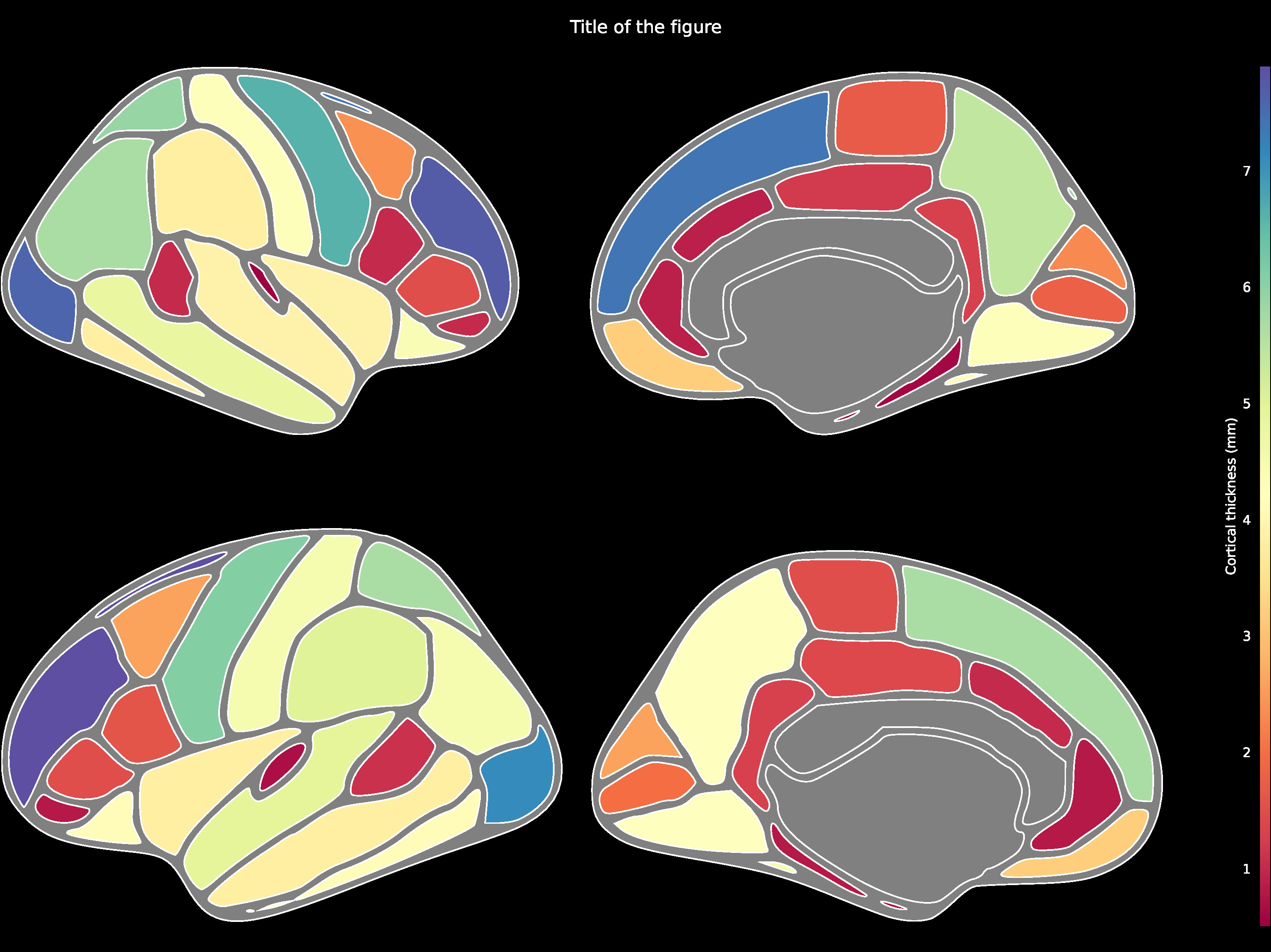

The comprehensive list of applicable regions can be found in this folder.

Subcortical regions (FreeSurfer aseg atlas)

data = {'Left-Lateral-Ventricle': 12289.6,
        'Left-Thalamus': 8158.3,
        'Left-Caudate': 3463.3,
        'Left-Putamen': 4265.3,
        'Left-Pallidum': 1620.9,
        '3rd-Ventricle': 1635.6,
        '4th-Ventricle': 1115.6,
        ...}

ax, plt_objs, cmap = ggseg.plot_aseg(data, cmap='Spectral',
                                     background='k', edgecolor='w', bordercolor='gray',
                                     ylabel='Volume (mm3)', title='Title of the figure')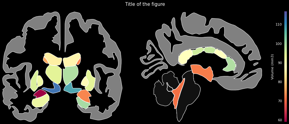

The comprehensive list of applicable regions can be found in this folder.

White-matter fiber tracts (Johns Hopkins University)

data = {'Anterior thalamic radiation L': 0.3004812598228455,
        'Anterior thalamic radiation R': 0.2909256815910339,
        'Corticospinal tract L': 0.3517134189605713,
        'Corticospinal tract R': 0.3606771230697632,
        'Cingulum (cingulate gyrus) L': 0.3149917721748352,
        'Cingulum (cingulate gyrus) R': 0.3126821517944336,
        ...}

ax, plt_objs, cmap = ggseg.plot_jhu(data, background='k', edgecolor='w', cmap='Spectral',
                                    bordercolor='gray', ylabel='Mean Fractional Anisotropy',
                                    title='Title of the figure')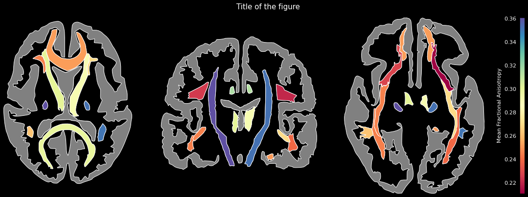

The comprehensive list of applicable regions can be found in this folder.

Hippocampal subregions

A hippocampus + entorhinal-cortex atlas is also bundled. Keys correspond to subregion files in ggseg/data/hippo: CA1, CA2, CA3, DG, EC (with LEC / MEC for the lateral and medial entorhinal subdivisions), sub, presub, parasub. The formation outline is used to size the figure and is not a data region.

data = {'CA1': 0.72,
        'CA2': 0.41,
        'CA3': 0.55,
        'DG':  0.83,
        'LEC': 0.30,
        'MEC': 0.38,
        'sub': 0.61,
        'presub': 0.48,
        'parasub': 0.52}

ax, plt_objs, cmap = ggseg.plot_hippo(data, cmap='viridis',
                                      background='k', edgecolor='w', bordercolor='gray',
                                      ylabel='Activation', title='Hippocampal subregions')

Plotting arrays inside regions

Instead of (or alongside) a single scalar per region, a region's value can be a 2D numpy array — it will be rendered as a heatmap, resampled to the region's bounding box and masked to the region outline. Scalars and arrays can be freely mixed in the same data dict, and the colormap bounds are computed across both.

import numpy as np
import ggseg

# Synthetic activation maps for two DK regions; the rest are flat scalars.
y, x = np.mgrid[0:50, 0:50]
data = {
    'precentral_left':   np.sin(x / 8) * np.cos(y / 8),
    'superiorfrontal_left': np.exp(-((x - 25)**2 + (y - 25)**2) / 200),
    'cuneus_left':       0.4,
    'lingual_left':      0.7,
}
ax, plt_objs, cmap = ggseg.plot_dk(data, cmap='viridis',
                                   background='w', edgecolor='k', bordercolor='gray')

The artist returned in plt_objs[region] is a matplotlib.patches.PathPatch for scalar values and a matplotlib.collections.QuadMesh (from ax.pcolormesh) for array values.

Animations

Because each plot_* returns the dict of patch / mesh artists, you can drive a matplotlib.animation.FuncAnimation by mutating them frame by frame — no need to redraw the atlas on every tick.

import numpy as np
import matplotlib.pyplot as plt
from matplotlib.animation import FuncAnimation
import ggseg

regions = ['precentral_left', 'superiorfrontal_left',
           'cuneus_left',     'lingual_left']
timeseries = {r: np.random.RandomState(i).randn(60).cumsum()
              for i, r in enumerate(regions)}

# Initial frame
data0 = {r: timeseries[r][0] for r in regions}
ax, plt_objs, cmap = ggseg.plot_dk(data0, cmap='viridis',
                                   background='w', edgecolor='k', bordercolor='gray',
                                   vminmax=[-5, 5])

def update(frame):
    norm = plt.Normalize(vmin=-5, vmax=5)
    for r in regions:
        plt_objs[r].set_facecolor(cmap(norm(timeseries[r][frame])))
    return list(plt_objs.values())

anim = FuncAnimation(ax.figure, update, frames=60, interval=80, blit=False)
anim.save('animation.gif', writer='pillow', fps=15)

For array-valued regions the artist is a QuadMesh, so use plt_objs[region].set_array(new_array.ravel()) inside update instead of set_facecolor.

Tests

The current development version of python-ggseg has a coverage rate close to 100%. The corresponding tests can be found in this folder.

Examples

A Jupyter Notebook with examples can be found there.