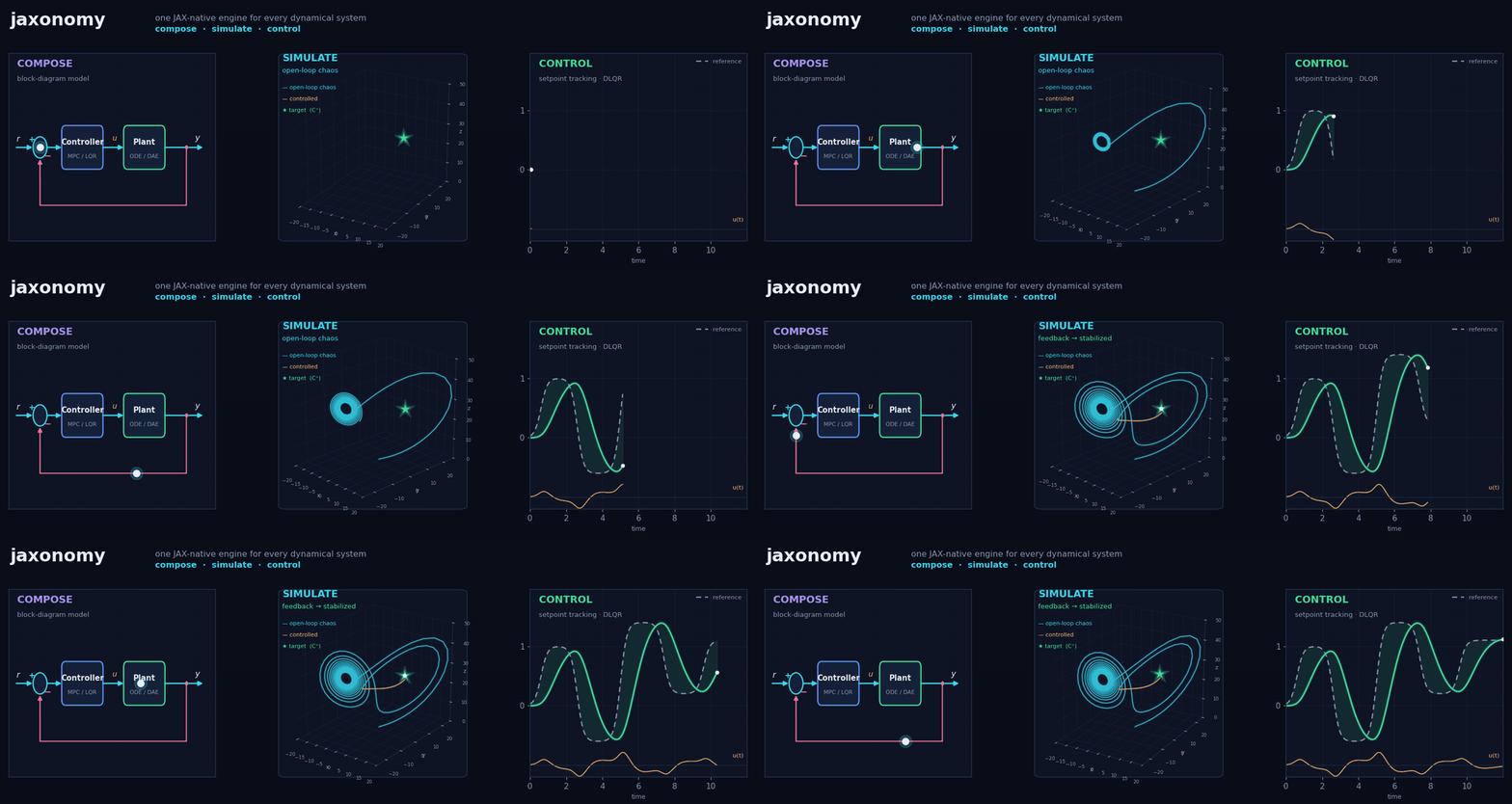
Differentiable simulation of hybrid dynamical systems — powered by JAX.



Block diagrams meet automatic differentiation. Model physical systems, close the loop with LQR/MPC/Kalman, and differentiate through everything.
Why JAX? · Install · Quick Start · Gallery · Examples · Docs
Every panel above is produced by jaxonomy.simulate on a model built from the library.
Jaxonomy is a Python framework for modeling, simulating, and optimizing hybrid dynamical systems — systems that combine continuous physics, discrete control laws, and event-driven logic in a single model. Every simulation runs on JAX, so it is JIT-compilable, batchable with vmap, and fully differentiable from end to end.
import jax.numpy as jnp
import jaxonomy as jx

# Double integrator: A, B, C, D define the plant; Q, R weight the LQR cost.
A, B = jnp.array([[0., 1.], [0., 0.]]), jnp.array([[0.], [1.]])
C, D = jnp.eye(2), jnp.zeros((2, 1))
Q, R = jnp.eye(2), jnp.array([[1.]])

builder = jx.DiagramBuilder()
plant      = builder.add(jx.library.LTISystem(A, B, C, D))
controller = builder.add(jx.library.LinearQuadraticRegulator(A, B, Q, R))
builder.connect(plant.output_ports[0],      controller.input_ports[0])
builder.connect(controller.output_ports[0], plant.input_ports[0])

diagram = builder.build()
results = jx.simulate(diagram, diagram.create_context(), (0.0, 10.0))Choosing JAX as the compute backbone unlocks capabilities that are impractical with NumPy-based simulators:
Traditional simulator          Jaxonomy / JAX
──────────────────────         ─────────────────────────────────────────
simulate(params)          →    jit(simulate)(params)          10–100× faster
for p in param_grid: …    →    vmap(simulate)(param_grid)     embarrassingly parallel
finite_diff_gradient(…)   →    grad(simulate)(params)         exact gradients, free
| Feature | SciPy / NumPy | Julia / DiffEq | Modelica | MathWorks¹ | Jaxonomy |
|---|---|---|---|---|---|
| Python-native | ✓ | ✗ | ✗ | ✗ | ✓ |
| JIT / code generation | ✗ | ✓ | ✓ (C++) | ✓ (C/C++) | ✓ |
| Full autodiff through ODE | ✗ | Partial | ✗ | Partial² | ✓ |
| Hybrid events & zero-crossing | Partial | ✓ | ✓ | ✓ | ✓ |
| Acausal / equation-based | ✗ | ✗ | ✓ | ✓ (Simscape) | ✓ |
| Block-diagram composition | ✗ | Partial | Partial | ✓ (Simulink) | ✓ |
| State-machine modeling | ✗ | ✗ | ✗ | ✓ (Stateflow) | ✓ |
| LQR / MPC / Kalman built-in | ✗ | Partial | Via libs | ✓ (Toolboxes) | ✓ |
| Neural ODE / SINDy | ✗ | ✓ | ✗ | ✗ | ✓ |
| Reduced-order modeling (balred / POD-DEIM / DMD / Koopman) | ✗ | Partial | ✗ | ✓ (Toolboxes) | ✓ |
| Batch / ensemble (vmap) | ✗ | ✗ | ✗ | ✗ | ✓ |
| Open-source (MIT) | ✓ | ✓ | Partial | ✗ | ✓ |
¹ Simulink + Simscape + Stateflow + Control System Toolbox · ² Via Simulink Design Optimization, no end-to-end AD
| Capability | What it enables |
|---|---|
| ⚡ JAX-native engine | JIT-compile simulations, run ensembles with vmap, differentiate through ODE solvers including event handling |
| 🔀 Hybrid dynamics + state machines | Continuous ODEs, periodic discrete updates, zero-crossing events, and StateMachineBuilder-authored finite state machines composed in one model. jax.grad flows through event times for hybrid trajectory optimisation. |
| 🔌 Acausal modeling | Modelica-inspired multi-domain components (electrical, mechanical, thermal, fluid, battery) with Pantelides index reduction and a BDF mass-matrix DAE solver |
| 🎯 Control & estimation | LQR (continuous, discrete, finite-horizon, LQG), linear MPC (native + OSQP), nonlinear MPC (shooting / transcription / Hermite-Simpson), Kalman / EKF / UKF / RLS / Luenberger, 2-DOF PID with classical tuning helpers |
| 🧮 Unit-aware wiring | Optional BusUnit annotations on ports and signals; the diagram compiler catches dimensional mismatches at build time instead of as silent runtime bugs |
| 🧠 Data-driven modeling | Neural ODEs, Universal Differential Equations, SINDy symbolic regression, neural-network blocks (MLP / PyTorch / TensorFlow / ONNX), differentiable lookup-table fitting, and statistical surrogates (Gaussian process, polynomial chaos, RBF) |
| 📉 Reduced-order modeling | jaxonomy.library.rom: linear MOR (balanced truncation, minreal, modal / residualization), POD–Galerkin with DEIM hyper-reduction, and data-driven operator ROM (DMD / DMDc / ERA, Koopman / eDMD lifted-linear predictors). One reduce(...) front door; every reduced model is a differentiable, simulatable block |
| 🎲 Uncertainty & sensitivity | First-class jaxonomy.uq workflow: Monte Carlo with parameter distributions, Latin Hypercube + quasi-Monte Carlo sampling, Sobol sensitivity decomposition, Morris screening |
| 🤝 FMI 2.0 / 3.0 interop | Import any FMI co-simulation FMU (ModelicaFMU) with mixed-type and array I/O; export a Jaxonomy diagram as a binary .fmu via build_fmu for use in Simulink / Dymola / OpenModelica |
| 🧩 150+ library blocks | Integrators, filters, state machines, look-up tables, coordinate transforms, container blocks, bus / mux family, stochastic sources, and more |
Requires Python 3.10+.
# Create and activate a virtual environment (recommended)
python -m venv .venv
source .venv/bin/activate        # Windows: .venv\Scripts\activate

# Install
pip install jaxonomy             # core
pip install jaxonomy[safe]       # + SciPy, Matplotlib, control, jaxopt
pip install jaxonomy[nmpc]       # + nonlinear MPC (requires IPOPT on PATH)
pip install jaxonomy[all]        # + everything
From source:
git clone https://github.com/machinavitalis/jaxonomy
cd jaxonomy
pip install -e .
CLI runner:
jaxonomy_cli run --model path/to/model.jsonA first simulation in a few lines — a custom block, built into a diagram, integrated through its ODE:
import jaxonomy as jx
import jax.numpy as jnp

# Van der Pol oscillator as a custom block
class VanDerPol(jx.LeafSystem):
    def __init__(self, mu=1.0, **kwargs):
        super().__init__(**kwargs)
        self.declare_dynamic_parameter("mu", mu)
        self.declare_continuous_state(
            default_value=jnp.array([0.0, 2.0]), ode=self._ode
        )
        self.declare_continuous_state_output(name="x")

    def _ode(self, time, state, *inputs, **params):
        x, mu = state.continuous_state, params["mu"]
        return jnp.array([x[1],  mu * (1 - x[0]**2) * x[1] - x[0]])

builder = jx.DiagramBuilder()
vdp = builder.add(VanDerPol(mu=2.0, name="vdp"))
diagram = builder.build()

results = jx.simulate(
    diagram, diagram.create_context(), (0.0, 20.0),
    options=jx.SimulatorOptions(buffer_length=4000),  # room for adaptive steps
    recorded_signals={"x": vdp.output_ports[0]},
)
# results.outputs["x"] → time-series of shape (T, 2)- Online docs & tutorials: py.jaxonomy.com
- Local docs:
pip install -r requirements.docs.txt mkdocs serve # → http://127.0.0.1:8000 - Example notebooks:
docs/examples/ - Scope notes: PINNs & PDE surrogates — classical PDE PINNs are out of scope; physics-informed dynamics learning (UDE / Neural DAE / Neural ODE / SINDy) is core.
Jaxonomy ships an MCP server that exposes the
engine as tools an AI agent can call directly — it can enumerate library blocks,
build and validate a model, run a simulation, fit parameters to data, and
linearize a system, then reason over the actual results. This is worth wiring up
if you drive Jaxonomy from an agent (Claude Desktop/Code, Cursor, …); if you're
writing Python by hand, the pip install above is all you need and you can skip
this.
pip install jaxonomy[mcp]Then register the server with your agent client. For Claude Desktop, add to
claude_desktop_config.json:
{
  "mcpServers": {
    "jaxonomy": {
      "command": "python",
      "args": ["-m", "jaxonomy.mcp.server"]
    }
  }
}
Use the interpreter where jaxonomy[mcp] is installed (or the jaxonomy-mcp
entry point). Full tool reference and configuration notes:
jaxonomy/mcp/README.md.

Jaxonomy is designed for hybrid systems — models where continuous physics interacts with instantaneous discrete resets. The bouncing ball is the canonical example: free-fall ODE interrupted by a collision event that reverses velocity.
The dynamics between bounces follow:
When the ball hits the ground (
import jaxonomy as jx
import jax.numpy as jnp

class BouncingBall(jx.LeafSystem):
    def __init__(self, g=9.81, e=0.8, **kwargs):
        super().__init__(**kwargs)
        self.declare_dynamic_parameter("g", g)
        self.declare_dynamic_parameter("e", e)
        # [height, velocity]
        self.declare_continuous_state(
            default_value=jnp.array([5.0, 0.0]), ode=self._ode
        )
        self.declare_continuous_state_output(name="state")

        # Zero-crossing: fires as height crosses zero from above
        self.declare_zero_crossing(
            guard=self._hit_ground,
            reset_map=self._bounce,
            direction="positive_then_non_positive",
        )

    def _ode(self, time, state, *inputs, **params):
        v = state.continuous_state[1]
        return jnp.array([v, -params["g"]])

    def _hit_ground(self, time, state, *inputs, **params):
        return state.continuous_state[0]  # guard on height

    def _bounce(self, time, state, *inputs, **params):
        x, v = state.continuous_state
        new_state = jnp.array([0.0, -params["e"] * v])
        return state.with_continuous_state(new_state)

builder = jx.DiagramBuilder()
ball = builder.add(BouncingBall(g=9.81, e=0.85, name="ball"))
diagram  = builder.build()
results  = jx.simulate(
    diagram, diagram.create_context(), (0.0, 8.0),
    recorded_signals={"state": ball.output_ports[0]},
)
Zero-crossing events are located with 40-step bisection on the solver's dense output polynomial — giving sub-microsecond temporal accuracy without user-specified tolerances.
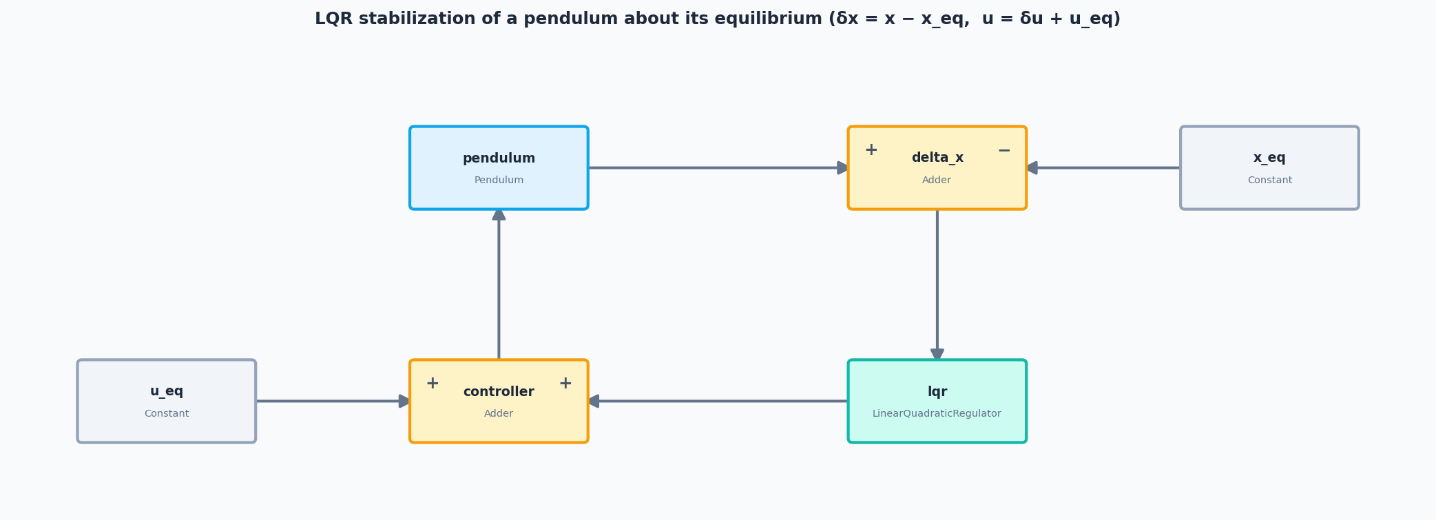
For a linearized pendulum with state
The Linear Quadratic Regulator minimizes infinite-horizon cost:
by solving the algebraic Riccati equation
import jaxonomy as jx
from jaxonomy.library import LTISystem, LinearQuadraticRegulator
import jax.numpy as jnp

g, L, m = 9.81, 1.0, 1.0
A = jnp.array([[0, 1], [g/L, 0]])
B = jnp.array([[0], [1 / (m * L**2)]])
C, D = jnp.eye(2), jnp.zeros((2, 1))

Q = jnp.diag(jnp.array([10.0, 1.0]))  # penalise angle more than rate
R = jnp.array([[0.1]])                 # control effort cost

builder    = jx.DiagramBuilder()
plant      = builder.add(LTISystem(A, B, C, D, name="pendulum"))
controller = builder.add(LinearQuadraticRegulator(A, B, Q, R, name="lqr"))

builder.connect(plant.output_ports[0],      controller.input_ports[0])
builder.connect(controller.output_ports[0], plant.input_ports[0])

diagram = builder.build()
context = diagram.create_context()

# Perturb the pendulum's initial angle by 15° (set one block's sub-state)
context = context.with_subcontext(
    plant.system_id,
    context[plant.system_id].with_continuous_state(jnp.array([jnp.pi / 12, 0.0])),
)

results = jx.simulate(
    diagram, context, (0.0, 5.0),
    recorded_signals={"x": plant.output_ports[0]},
)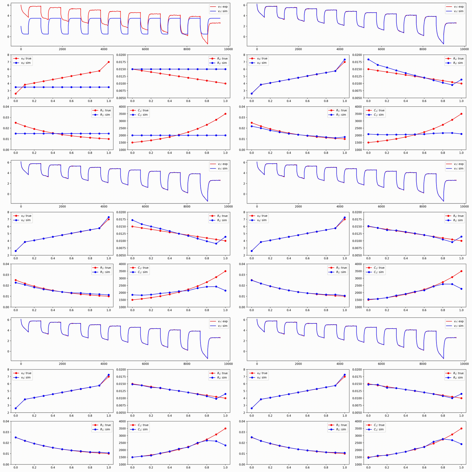
Jaxonomy can differentiate through complete simulations to fit model parameters to data — no finite-difference approximations, no hand-written adjoint code. Here we recover a spring–damper's stiffness and damping by differentiating the whole rollout and descending with Optax:
import jax
import jax.numpy as jnp
import optax
import jaxonomy as jx

class SpringDamper(jx.LeafSystem):
    def __init__(self, k=1.0, c=0.3, **kwargs):
        super().__init__(**kwargs)
        self.declare_dynamic_parameter("k", k)
        self.declare_dynamic_parameter("c", c)
        self.declare_continuous_state(
            default_value=jnp.array([1.0, 0.0]), ode=self._ode
        )

    def _ode(self, time, state, *inputs, **params):
        x, v = state.continuous_state
        return jnp.array([v, -params["k"] * x - params["c"] * v])

sd   = SpringDamper(name="sd")
opts = jx.SimulatorOptions(enable_autodiff=True, max_major_steps=200)

def final_state(theta):                       # theta = {"k": ..., "c": ...}
    ctx = sd.create_context()
    ctx.parameters["k"], ctx.parameters["c"] = theta["k"], theta["c"]
    res = jx.simulate(sd, ctx, (0.0, 1.5), options=opts)
    return res.context.continuous_state       # differentiable final [x, v]

target = jax.lax.stop_gradient(final_state({"k": 4.0, "c": 0.5}))  # "measured"
loss   = lambda theta: jnp.sum((final_state(theta) - target) ** 2)

theta   = {"k": 1.0, "c": 0.1}
opt     = optax.adam(2e-1)
state   = opt.init(theta)
grad_fn = jax.jit(jax.grad(loss))             # gradient through the ODE solver
for _ in range(300):
    updates, state = opt.update(grad_fn(theta), state)
    theta = optax.apply_updates(theta, updates)
# theta → {"k": 4.00, "c": 0.50}
jax.grad(loss) flows back through every ODE step automatically, so the same recipe scales to battery ECMs (above), powertrains, or any parametric model — and jaxonomy.optimization wraps it in a higher-level Optimizable API when you want bounds, transforms, and constraints.
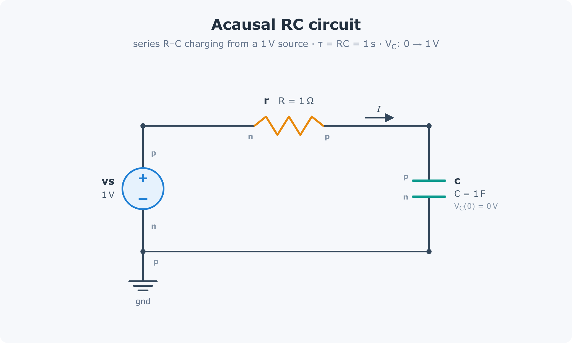
Jaxonomy includes a Modelica-inspired acausal modeling layer for multi-domain physical systems. You describe component connections symbolically; the compiler automatically derives the governing DAE, reduces its index, and emits a LeafSystem ready to drop into any diagram.
RC circuit with initial conditions:
import jaxonomy as jx
from jaxonomy.acausal import AcausalCompiler, AcausalDiagram, EqnEnv
from jaxonomy.acausal import electrical as elec

ev = EqnEnv()
ad = AcausalDiagram()

vs  = elec.VoltageSource(ev, name="vs", v=1.0)
r   = elec.Resistor(ev,      name="r",  R=1.0)
c   = elec.Capacitor(ev,     name="c",  C=1.0,
                              initial_voltage=0.0, initial_voltage_fixed=True)
gnd = elec.Ground(ev,        name="gnd")

ad.connect(vs, "p", r,  "n")
ad.connect(r,  "p", c,  "p")
ad.connect(c,  "n", vs, "n")
ad.connect(vs, "n", gnd, "p")

compiler = AcausalCompiler(ev, ad)
rc_block = compiler()         # → LeafSystem, JIT-compiled ODE

builder = jx.DiagramBuilder()
builder.add(rc_block)
diagram = builder.build()
results = jx.simulate(diagram, diagram.create_context(), (0.0, 5.0))
The same pipeline handles multi-domain systems — an electro-mechanical actuator connecting electrical, rotational, and translational domains compiles to a single optimized system.
Available acausal domains: electrical · rotational · translational · thermal · fluid
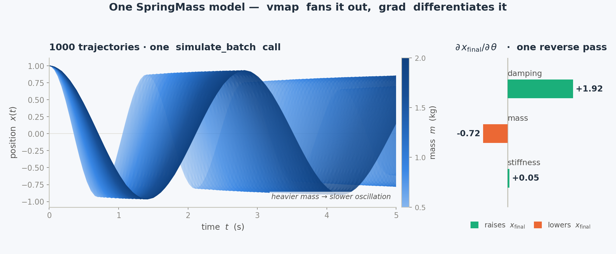
Because jax.grad, jax.jit, and jax.vmap all compose with simulate, you get powerful workflows with minimal boilerplate:
import jax
import jax.numpy as jnp
import jaxonomy as jx

class SpringMass(jx.LeafSystem):
    def __init__(self, mass=1.0, damping=0.1, stiffness=10.0, **kwargs):
        super().__init__(**kwargs)
        self.declare_dynamic_parameter("mass", mass)
        self.declare_dynamic_parameter("damping", damping)
        self.declare_dynamic_parameter("stiffness", stiffness)
        self.declare_continuous_state(
            default_value=jnp.array([1.0, 0.0]), ode=self._ode
        )
        self.declare_continuous_state_output(name="x")

    def _ode(self, time, state, *inputs, **params):
        x, v = state.continuous_state
        a = -(params["stiffness"] * x + params["damping"] * v) / params["mass"]
        return jnp.array([v, a])

# ── Sensitivity: ∂(final position)/∂(all parameters) in one reverse pass ─────
plant = SpringMass(name="plant")
grad_opts = jx.SimulatorOptions(enable_autodiff=True, max_major_steps=200)

def final_position(theta):
    ctx = plant.create_context()
    for name, value in theta.items():
        ctx.parameters[name] = value
    res = jx.simulate(plant, ctx, (0.0, 5.0), options=grad_opts)
    return res.context.continuous_state[0]

grads = jax.grad(final_position)({"mass": 1.0, "damping": 0.1, "stiffness": 10.0})

# ── Monte Carlo ensemble: 1000 trajectories over a mass sweep (vmap) ─────────
builder = jx.DiagramBuilder()
plant_b = builder.add(SpringMass(name="plant"))
diagram = builder.build()

results = jx.simulate_batch(
    diagram, t_span=(0.0, 5.0),
    param_batches={"plant.mass": jnp.linspace(0.5, 2.0, 1000)},
    options=jx.SimulatorOptions(math_backend="jax", max_major_steps=200),
    recorded_signals={"x": plant_b.output_ports[0]},
)
# results.outputs["x"] shape: (1000, T, 2)Over 150 built-in blocks covering the full signal-processing and control toolkit. A representative slice — not exhaustive:
| Category | Blocks |
|---|---|
| Sources | Constant, Step, Ramp, Chirp, Pulse, Sawtooth, Clock, DataSource |
| Stochastic | RandomNumber, UniformRandomNumber, WhiteNoise, BandLimitedNoise, PRBS, RandomSource — all support with_key for independent noise streams under vmap |
| Arithmetic & nonlinearities | Adder, Gain, Product, Abs, Power, Trigonometric, Saturate / SoftSaturate, DeadZone, RateLimiter / SoftRateLimiter, Quantizer, Backlash |
| Continuous dynamics | Integrator, Derivative, TransferFunction, LTISystem, PID / PIDContinuous |
| Discrete dynamics | IntegratorDiscrete, UnitDelay, FilterDiscrete, LowPassDiscrete, LeadLag, Notch, PIDDiscrete, PIDController2DOF, Decimator, RateTransition |
| Routing, buses, matrix | Mux / Demux, BusCreator / BusSelector / BusUpdate (with BusUnit annotations), Slice, Stack, Switch / MultiPortSwitch, IfThenElse, MatrixMultiplication, MatrixInversion, DotProduct, CrossProduct |
| Logic & state machines | TruthTable, LogicalOperator, Comparator, Relay, EdgeDetection, StateMachine (authored via StateMachineBuilder DSL) |
| Lookup tables | LookupTable1d / LookupTable2d / LookupTableND, Prelookup / InterpolationUsingPrelookup, TableSearch — all differentiable and fittable from data via fit_lookup_table_* |
| Delays & containers | TransportDelay, VariableTransportDelay, EnabledSubsystem, TriggeredSubsystem, ForEach, Conditional |
| Control | LinearQuadraticRegulator / DiscreteTimeLinearQuadraticRegulator / FiniteHorizonLinearQuadraticRegulator / LinearQuadraticGaussian, LinearDiscreteTimeMPC (native + LinearDiscreteTimeMPC_OSQP), DirectShootingNMPC / DirectTranscriptionNMPC / HermiteSimpsonNMPC |
| Estimation | KalmanFilter, ExtendedKalmanFilter, UnscentedKalmanFilter, InfiniteHorizonKalmanFilter, RecursiveLeastSquares, AugmentedStateEKF, Luenberger |
| Physics & coordinates | CoordinateRotation, RigidBody, BatteryCell |
| ML / Data | MLP (Equinox), Sindy, PyTorch, TensorFlow, ONNX / ONNXJax |
| ROM & surrogates | reduce(...) → ReducedOrderModel; linear MOR (balred / minreal / modal_truncation / residualize), galerkin_reduce + deim (POD–DEIM), dmd / dmdc / era, DMDForecaster / KoopmanPredictor, and surrogate blocks GaussianProcess / PolynomialChaos / RadialBasisSurrogate |
| Interop | ModelicaFMU (FMI 2.0 / 3.0 co-simulation import) + FMU export via build_fmu; MuJoCo / MJX; Ros2Publisher / Ros2Subscriber; QuanserHAL; PyTwin |
| Custom | CustomPythonBlock, CustomJaxBlock for user-authored algorithms with persistent per-instance state |
Custom blocks are first-class beyond the wrappers above: subclass LeafSystem, declare ports and states, and your block integrates with the full framework including JIT, autodiff, and event detection.
A Jaxonomy model is a Diagram — a directed graph of interconnected blocks. Blocks (LeafSystem) declare ports, continuous/discrete states, and event guards. The simulator orchestrates ODE integration, discrete updates, and event detection automatically.
graph LR
    subgraph Diagram["DiagramBuilder.build()"]
        direction LR
        r[/"r(t)\nReference"/] --> sum(("Σ"))
        sum -->|"e(t)"| ctrl["Controller\nLQR · MPC · PID"]
        ctrl -->|"u(t)"| plant["Plant\nLTI · Nonlinear · Acausal"]
        plant -->|"x(t)"| obs["State Estimator\nKalman · EKF · UKF"]
        obs --> sum
        plant -->|"y(t)"| out[/"y(t)\nOutput"/]
    end

    style Diagram fill:#f5f8ff,stroke:#4a6fa5,stroke-width:2px
    style ctrl fill:#dbeafe,stroke:#2563eb
    style plant fill:#dcfce7,stroke:#16a34a
    style obs fill:#fef9c3,stroke:#ca8a04
The JAX backend sits underneath every simulation, giving you a clean Python API backed by XLA compilation:
graph TD
    A["Python API\nDiagram · LeafSystem · simulate()"] --> B["JAX Backend\nJIT · vmap · grad"]
    B --> C1["Dopri5\nAdaptive RK45\nnon-stiff ODEs"]
    B --> C2["BDF\nImplicit solver\nstiff systems"]
    B --> C3["Event Handler\nZero-crossing\nbisection"]

    style A fill:#e0f2fe,stroke:#0284c7
    style B fill:#fdf4ff,stroke:#9333ea
    style C1 fill:#f0fdf4,stroke:#16a34a
    style C2 fill:#f0fdf4,stroke:#16a34a
    style C3 fill:#f0fdf4,stroke:#16a34a
Jaxonomy is the engine at the base of a three-package stack. Each package is its own repository, MIT-licensed, and depends only on the package(s) above it:
- Jaxonomy — this package. The general-purpose, JAX-native simulation engine for hybrid dynamical systems. Not robotics-specific; depends on nothing else in the stack.
- Jaxterity — the robotics layer built on top of Jaxonomy: URDF/MJCF import, MJX-backed articulated dynamics, calibrated actuators/sensors, system identification, and whole-body control. Imports Jaxonomy; never re-implements its primitives.
- Jaxility — the deployment artifact factory: compiles a calibrated robot to embedded C for Arm SoCs (Cortex-A / Cortex-M) with a signed attestation manifest. Consumes Jaxterity.
The boundary rule: anything useful to controls engineers outside robotics (HVAC, battery, aerospace, energy) belongs in Jaxonomy; anything specific to joints, actuators, contacts, and kinematic chains belongs in Jaxterity; embedded codegen, targets, and attestation belong in Jaxility.
What Jaxonomy does not yet do (or does only partially) is tracked in
KNOWN_GAPS.md — the public inverse of the internal evidence
ledger in CLAIMS.md.
Released under the MIT License from version 2.2.0 onward.
Derived from the MIT-licensed open-source package pycollimator by Collimator, Inc.