Cuda Parallel Marching Blocks

cupmb extracts the zero level set of a scalar field on the GPU from Python: root finding in 1D, marching squares in 2D and marching cubes in 3D. It implements the Parallel Marching Blocks (PMB) algorithm, see Parallel Marching Blocks: A Practical Isosurfacing Algorithm for Large Data on Many-Core Architectures.

• Indexed meshes: vertices are shared between the simplices of a block, no triangle soup.
• Your scalar field, compiled: an analytic CUDA device function or a sampled array, compiled at runtime with NVRTC and cached on disk.
• Skip empty space: an optional block predicate (for instance with interval or affine arithmetic) discards the blocks that cannot contain the surface, the cost then scales with the surface instead of the volume.
• Built for real time: autotuned block sizes, a single device to host copy per call, no recompilation when the grid size or the extra parameters change, output buffers can be OpenGL buffers.
• CuPy or PyCUDA backends.

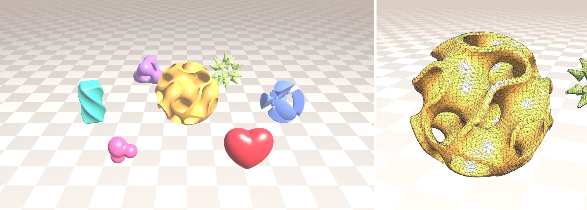
Scene of 08_levelset.py meshed at N = 1024 (2.8 M triangles), and the wireframe of the gyroid ball at N = 192.

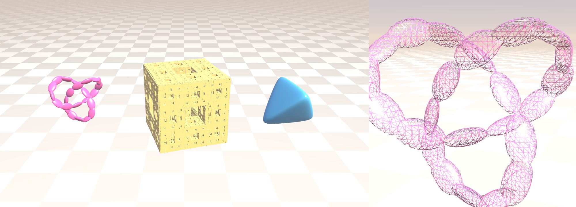
Level sets written with Eigen matrices (09_eigen_levelset.py) meshed at N = 2048 (15.5 M triangles), and the wireframe of the trefoil knot at N = 256.

Performance

Median time of a call on a RTX 5090 (CUDA 12.9, CuPy 13.6, single precision, outputs kept on the device), as reported by the benchmarks of the examples:

Example	Grid	Output	Without predicate	With predicate
07_predicate.py	2048³	27.4 M triangles	44.5 ms	4.1 ms
08_levelset.py (animated scene)	5120 × 1463 × 4568	60.5 to 71.0 M triangles	241.9 ms	91.1 ms
09_eigen_levelset.py (Eigen)	2560 × 872 × 918	19.8 to 37.1 M triangles	192.9 ms	61.3 ms
10_gamma.py (1D)	2³²	4.08 M roots	570 ms	227 ms

Requirements

• Linux, NVIDIA GPU and driver.
• Python >= 3.10.
• CUDA 12.x (tested with CUDA 12.9 on a sm_120 GPU). The CUDA 13 cupy wheel (cupy-cuda13x) can be selected with the cupy13 extra.
• One of the two backends: CuPy (default) or PyCUDA.
• Header only device libraries: trove (git submodule, shipped with the package) and cusvna (cusvna package on PyPI, installed as a dependency).
• Examples 7 to 9 also include autodiff (CUDA fork) and example 9 eigen-nvrtc (Eigen patched for NVRTC), both git submodules that are only needed by the examples and not shipped with the package.

Getting started

cupmb is available on PyPI, pick a backend extra (cupy12, cupy13 for CUDA 13 or pycuda):

python3 -m pip install "cupmb[cupy12]"

To run the examples, clone the repository with its submodules:

git clone --recursive https://github.com/keckj/cupmb.git
cd cupmb
python3 -m venv .venv && source .venv/bin/activate
python3 -m pip install ".[cupy12,examples]"  # cupmb, its CuPy backend and the dependencies of the examples
python3 examples/00_simple.py                # meshes a sphere and displays it with trimesh

If the repository was cloned without --recursive, run git submodule update --init --recursive before installing.

Available extras, combine them with commas:

Extra	Content
cupy12	CuPy backend for CUDA 12 (cupy-cuda12x)
cupy13	CuPy backend for CUDA 13 (cupy-cuda13x)
pycuda	PyCUDA backend (pycuda, cuda-python for NVRTC)
gl	Cuda/OpenGL interoperability (cuda-python, PyOpenGL)
examples	Dependencies of the examples (trimesh, open3d, matplotlib, glfw, ...)
test	Test suite (pytest, scipy)
dev	Test suite, build, pre-commit, black, ruff, scikit-image

All the dependencies of the examples (both backends included) can also be installed with python3 -m pip install -r requirements_examples.txt.

Minimal usage

from cupmb import ParallelMarchingBlocks

fdef = r"""
namespace cupmb {
    template <typename T, typename I, I dim>
    __device__ __forceinline__ T scalar(
            const trove::array<T,dim>& p,
            const trove::array<I,dim>& i) {
        const T& x = trove::get<0>(p);
        const T& y = trove::get<1>(p);
        const T& z = trove::get<2>(p);
        return x*x + y*y + z*z - T(0.45)*T(0.45);
    }
}
"""
pmb = ParallelMarchingBlocks(3, fdef, N=64, x0=-0.5, L=1.0)
V, I = pmb(to_numpy=True)  # vertices (nv, 3) float32, triangles (nt, 3) uint32

• The scalar function receives the position p and the integer coordinates i of each grid point. The grid size is a kernel argument and not a template parameter (former template <typename T, typename I, I dim, I... N> signatures are still accepted, N is then empty).
• Without to_numpy=True the output buffers stay on the device. When the zero level set is empty, V and I are None.
• Verbosity is controlled by the CUPMB_LOGLEVEL environment variable (DEBUG, INFO, WARNING, ...).

Features

Output

• PMB outputs an indexed mesh: vertices are shared between the simplices of a block, no triangle soup as with other marching cubes algorithms. Vertices lying on the faces shared by two blocks are duplicated, weld them by position if you need a fully connected mesh.
• 1D (zero crossings, single vertex simplices), 2D (marching squares, segments) and 3D (marching cubes, triangles) support, single or double precision for vertices. In 1D, V and I have shape (n, 1) and simplex k references vertex k, vertices are never duplicated on block boundaries.
• uint32 or uint64 simplex indices.
• Consistently oriented simplices: normals point from negative to positive scalar values (along the gradient). Triangles are counterclockwise when seen from the positive side (closed surfaces have a positive signed volume) and segments are counterclockwise around negative regions (positive signed area). 1D simplices (single vertices) carry no orientation, the normal is the sign of the derivative and can be computed as a vertex property.
• Custom user defined vertex properties (normals, colors, ...) computed on the GPU alongside the vertices.
• Vertices and simplices are stored as array of structures, vector loads and stores are optimized with trove.

Input

• The scalar field can be analytic (function computed at runtime on the GPU) or stored in an array/texture. The sampled scalar field can be exported (export_scalar_field=True), it is stored x-fastest and indexed as S[iz,iy,ix] (shape N[::-1]+1, S[iy,ix] in 2D as expected by matplotlib.imshow or contour).
• User provided extra kernel parameters (constants or Python callables evaluated at each call).
• Dynamic domains (axis-aligned bounding box) and dynamic kernel parameters.

Performance

• Runtime KD-tree-pyramid domain decomposition (binary tree in 1D, quadtree in 2D and octtree in 3D) from analytic block predicates (pdef). Predicates can be computed with range analysis by using interval arithmetic or affine arithmetic, for instance with the cusvna headers (#include <cusvna/af1.cuh>, requires enable_cuda_std_lib=True).
• Once the buffers are large enough, a call performs a single device to host copy: kernels read the active block, vertex and simplex counts from device counters and grids are sized from the buffer capacities. When a count exceeds a capacity, the buffers are reallocated and the kernels launched again step by step.
• Low memory consumption with user configurable allocation policies (and possibly user provided buffers).

Integration

• Compatible with both CuPy and PyCUDA backends.
• Cuda/OpenGL interoperability: vertices and simplices can be written directly into OpenGL buffers.

Kernel cache

Kernels are compiled at runtime with NVRTC for each configuration (dimension, block sizes, types, user code, ...), autotuning compiles one module per candidate block size. The grid size is a kernel argument: changing N does not trigger any compilation. Compiled modules are cached on disk so that subsequent runs skip the compilation (example 8 starts in about 1.5 s instead of 25 s):

• the cache directory is $CUPMB_CACHE_DIR/kernels, it defaults to ~/.cache/cupmb/kernels ($XDG_CACHE_HOME/cupmb/kernels), see cupmb.kernel_cache_dir();
• set CUPMB_DISABLE_KERNEL_CACHE=1 to disable it and call cupmb.clear_kernel_cache() (or remove the directory) to clear it;
• entries are keyed by the cupmb version, the backend and its NVRTC version, the device compute capability, the kernel source code, the build options and the content of the cupmb kernel headers (including trove and cusvna). Headers included from other directories through extra_build_options are not part of the key: clear the cache when they change.

Examples

All the examples run with python3 -m pip install ".[cupy12,examples]", some of them need an additional extra:

Example	Dim	Topic	Extra
00_simple.py	3D	Analytic sphere, mesh displayed with trimesh
01_animation.py	3D	Extra kernel parameter, mesh recomputed at each frame
02_normals.py	3D	Normals as a vertex property
03_glinterop_cupy.py	3D	Cuda/OpenGL interoperability with CuPy	gl
03_glinterop_pycuda.py	3D	Cuda/OpenGL interoperability with PyCUDA	pycuda
04_isolines.py	2D	Marching squares compared to matplotlib.contour
05_moving_sphere.py	3D	Extra parameters given as Python callables
06_moving_bbox.py	3D	Dynamic bounding box
07_predicate.py	3D	Block predicate benchmark (affine arithmetic)
08_levelset.py	3D	Real time meshing of an animated scene, OpenGL viewer	gl
09_eigen_levelset.py	3D	Level sets written with Eigen matrices, OpenGL viewer	gl
10_gamma.py	1D	Root finding on 2³² cells

• 00_simple.py This simple example will show you how to execute the marching cubes algorithm to find the zero levelset of a scalar field representing a sphere. The scalar field is defined as $\phi(x,y,z) = x^2 + y^2 + z^2 - r^2$ where $r=0.45$ is a constant. The function is analytic and implemented directly as a device function. The default bounding box is $[0,1]^3$ so we offset it by $x_0=-0.5$ to find the zeros for $(x,y,z) \in [-0.5,+0.5]^3$. The output mesh (vertices V, simplices I) is copied to the host (numpy arrays) and is then displayed by using the trimesh module. Parameter N controls the resolution of the marching cubes algorithm.
• 01_animation.py Sphere with a radius given as an extra kernel parameter (extra_params=[("r", "T")], passed as pmb(r=...)), the mesh is recomputed at each frame and displayed with open3d.
• 02_normals.py User defined vertex properties (VertexProperty): normals are computed on the GPU alongside the vertices and used for shading in an open3d GUI.
• 03_glinterop_cupy.py, 03_glinterop_pycuda.py Cuda/OpenGL interoperability: vertices and simplices are written directly into OpenGL buffers (no host round trip) and rendered with glfw/PyOpenGL (lock_buffer/replace_buffer), with the CuPy and PyCUDA backends respectively. The PyCUDA version requires PyCUDA to be built with OpenGL support (pycuda.gl), which is not the case of a default python3 -m pip install pycuda.
• 04_isolines.py Marching squares in 2D: isolines of an analytic scalar field, the sampled scalar field is exported (export_scalar_field=True) and displayed with matplotlib, the cupmb segments (red) are compared to matplotlib.contour (black).
• 05_moving_sphere.py Extra kernel parameters (ExtraParameter) given as Python callables that are evaluated before each call, here the center of a moving sphere.
• 06_moving_bbox.py Dynamic domain: the bounding box follows the moving sphere through a user provided update_bbox callback.
• 07_predicate.py Benchmark of the block predicate based domain decomposition against the naive block extraction, the predicate is written with cusvna affine arithmetic. Run python3 examples/07_predicate.py --help for the options (-N grid size, --rigor autotuning rigor, --runs), large grids require a lot of device memory. The mesh is then displayed with open3d at a lower resolution (--display-N, default 512, --no-display to disable), shaded with exact normals computed on the GPU as a vertex property by forward automatic differentiation of the same template (autodiff Real numbers).
• 08_levelset.py Real time meshing of the animated scene of the last cusvna example (gyroid ball surrounded by a ring of heart, Kummer, Barth, tetrahedral, twisted box and metaballs level sets): the shapes are written once as templates evaluated on floats for the scalar field, on cusvna affine forms for the block predicate and on autodiff numbers for the exact normals, vertices, triangles, normals and colors are written directly into OpenGL buffers and rendered with glfw/PyOpenGL. The predicate scales with the surface instead of the volume, it is slower at small N and pays off at high resolution.
  • Controls (shown in an overlay when pyimgui is installed, logged at startup otherwise): SPACE pause, +/- (or UP/DOWN) animation speed, *// (or PAGE UP/PAGE DOWN) multiply or divide the resolution by two between 64 and 4096 cells along x, W wireframe, mouse to rotate and zoom, Q/ESC quit. The viewer uses a power of two number of cells on each axis, the domain is extended around the scene. When the resolution changes, the marching blocks are rebuilt with the ESTIMATE autotuning rigor, the grid size being a kernel argument the kernels are not recompiled.
  • Options: -N grid size (default 2048 for the viewer, 5120 for the benchmark), --no-predicate, --rigor autotuning rigor, --frames number of frames, --no-display headless benchmark with and without predicate (median meshing times, triangle counts are checked to be identical), --time animation time of the first frame, --size window size (WIDTHxHEIGHT), --wireframe, --screenshot FILE saves the first frame and quits (the figures of this README).
• 09_eigen_levelset.py The scene of the Eigen example of cusvna (Menger sponge as a kaleidoscopic iterated function system, spectrahedron, ellipsoidal beads along a trefoil knot) with the viewer, benchmark and options of 08_levelset.py. The shapes are written with Eigen vectors and matrices (rotations, quaternions, Householder reflections, determinants, quadratic forms) of floats, cusvna AF1 affine forms and autodiff numbers, Eigen being compiled by NVRTC from the eigen-nvrtc submodule. Only AF1 forms can be Eigen scalars: the type of an AA form changes with each nonlinear operation.
• 10_gamma.py Marching blocks in 1D: root finding on a very fine grid ($N=2^{32}$ cells on $[2^{-8}, 10^6]$ by default, 64 bit indices). The gamma function has no zero, the example finds instead the solutions of $\Gamma(x)=e^{k\pi}$, $k \in \mathbb{Z}$, i.e. the zeros of $\sin(\ln\Gamma(x))$ for $x>0$, with a cusvna affine arithmetic predicate (binary tree), about 4 million roots. The roots are checked against a host bisection (vectorized with the Stirling series of $\ln\Gamma$) and displayed with matplotlib (--no-plot to disable).

Testing

python3 -m pip install ".[cupy12,test]"
python3 -m pytest            # requires a CUDA device, GPU tests are skipped otherwise
python3 -m pytest --runslow  # also runs the large grid and large index tests (several GB of device memory)

If scikit-image is installed (dev extra), the 3D meshes are also cross-checked against skimage.measure.marching_cubes.

Development

python3 -m pip install -e ".[cupy12,dev]"
pre-commit install
python3 -m build  # sdist and wheel in dist/

License

cupmb is released under the MIT License. The device header libraries keep their own licenses: trove (BSD 3-clause, NVIDIA, shipped with the package) and cusvna (MIT). The examples also use autodiff (MIT) and Eigen (MPL 2.0).