🎨 3D Hilbert Depth Colormap

Give your depth estimation a fancy new colormap! Here you'll find an implementation of a bijective metric depth $\leftrightarrow$ RGB mapping along a 3D Hilbert cube walk, as used in the Vision Banana 🍌 paper [1].

📦 Installation

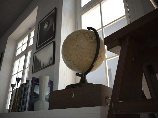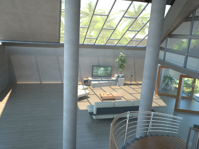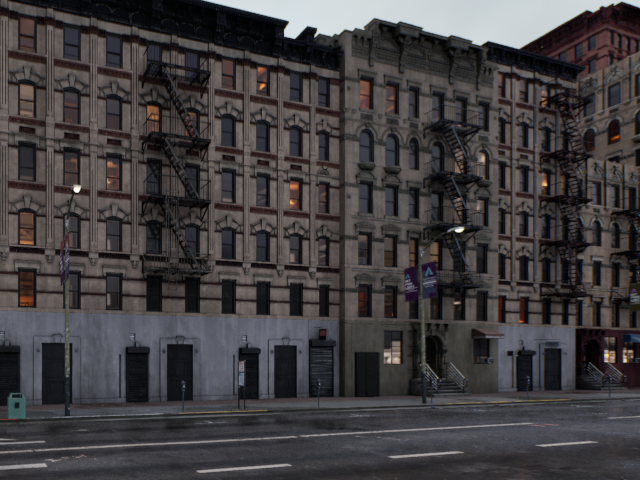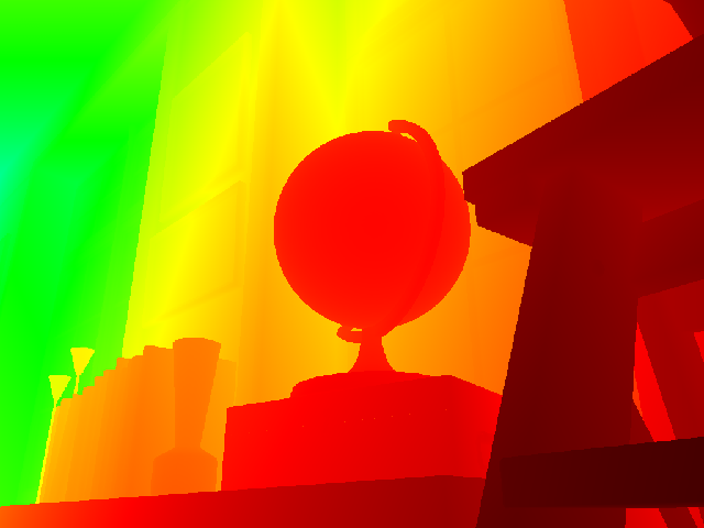From PyPI:

pip install hilbertmap

From source:

git clone https://github.com/massimilianoviola/hilbertmap
cd hilbertmap
pip install -e .

🛠️ Usage

Direct encoding/decoding

import numpy as np
from hilbertmap import depth_to_rgb, rgb_to_depth

depth = np.load("depth.npy")          # (H, W) float meters
rgb   = depth_to_rgb(depth)           # (H, W, 3) float in [0, 1]
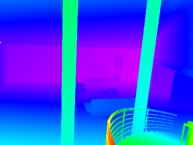
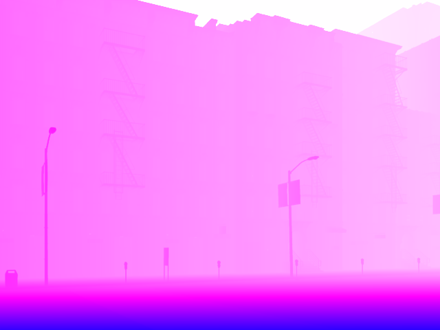
back  = rgb_to_depth(rgb)             # (H, W) recovered meters

Because the utility of accurate metric depth for nearby image content is generally higher than that of distant content, the default parameters $\lambda = -3$, $c = 10/3$ make the cube walk most sensitive in the first few meters and saturate beyond ~40 m. This behavior can be tuned by changing the parameters to get more meaningful color variation on deep outdoor scenes.

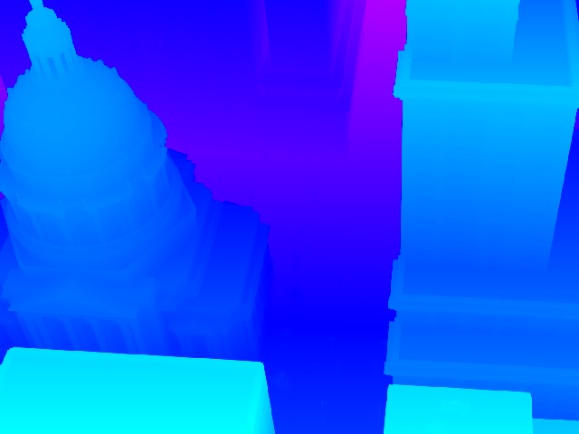
rgb  = depth_to_rgb(depth, lam=-4.0, c=120.0)  # tuned for long-range outdoor scene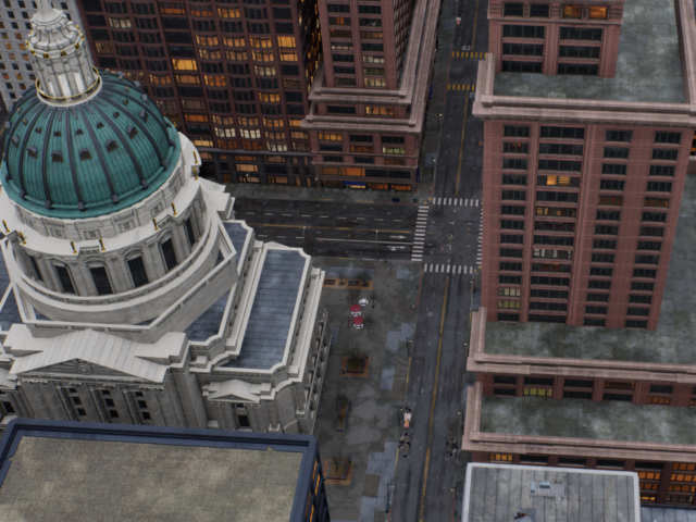

To swap the Barron transform (see explanation below) for a different normalization (linear, log, etc.), use the cube walk primitives directly. hm.walk maps a scalar in $[0, 1]$ to RGB along the cube path, and hm.project is its inverse:

f    = np.clip((depth - vmin) / (vmax - vmin), 0.0, 1.0)  # any forward map from [0, inf) to [0, 1]
rgb  = hm.walk(f)

back = vmin + (vmax - vmin) * hm.project(rgb)             # invert to recover depth

Visualization with matplotlib

import matplotlib.pyplot as plt
import hilbertmap as hm

im = plt.imshow(depth, cmap=hm.cmap(), norm=hm.Norm())
hm.colorbar(im, label="depth (m)")
plt.show()

hm.Norm applies the fixed power transform (same depth $\to$ same color across images). With this, hm.colorbar spans only the cmap subset the data actually covers.

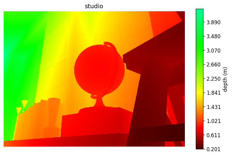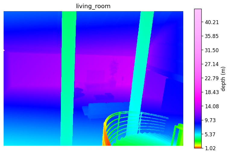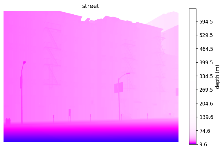In addition, transform params can be tuned as in direct encoding:

im = plt.imshow(depth, cmap=hm.cmap(), norm=hm.Norm(lam=-4.0, c=120.0))  # global, long-range outdoor
hm.colorbar(im, label="depth (m)")
plt.show()

Note that passing vmin / vmax to hm.Norm does not rescale the mapping, only the displayed colorbar range:

im = plt.imshow(depth, cmap=hm.cmap(), norm=hm.Norm(vmin=2.0, vmax=10.0))  # same global mapping, colorbar rescaled
hm.colorbar(im, label="depth (m)")  # <- this now shows [2, 10]
plt.show()

For per-image rescaling without the power transform, pair hm.cmap() with a standard matplotlib normalizer or simply omit it. This is the default behavior of other matplotlib colormaps.

Omit the normalizer to autoscale linearly to the data's min and max:

im = plt.imshow(depth, cmap=hm.cmap())  # linear, autoscaled to min/max, covering full cmap from black to white
hm.colorbar(im, label="depth (m)")
plt.show()

Or pass vmin and vmax for a fixed range:

im = plt.imshow(depth, cmap=hm.cmap(), vmin=0.0, vmax=80.0)               # linear, fixed range
# im = plt.imshow(depth, cmap=hm.cmap(), norm=plt.Normalize(0.0, 80.0))   # equivalent
hm.colorbar(im, label="depth (m)")
plt.show()

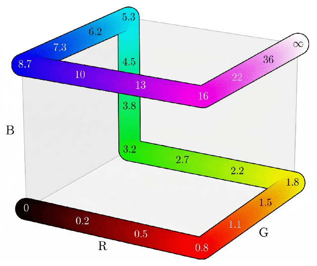
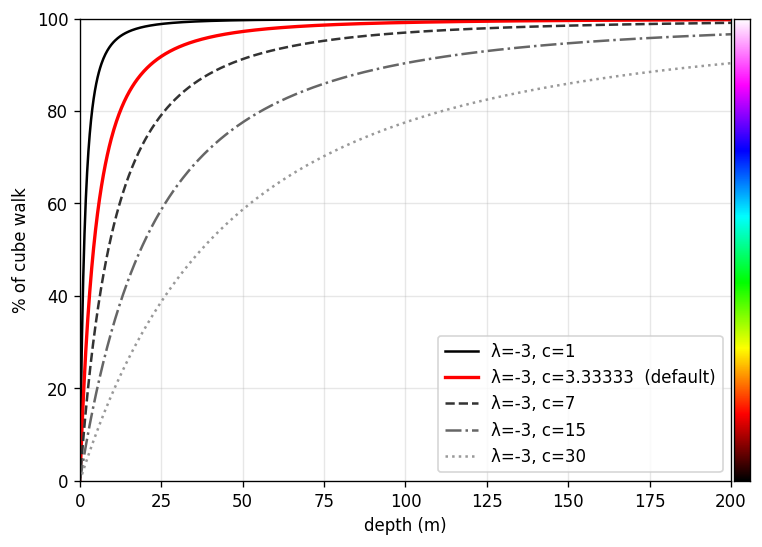
🧭 How it works

The seven-edge Hamiltonian path on the RGB cube (left) carries depth values from black at zero to white at infinity. The shape parameters $\lambda$ and $c$ produce different saturation curves (right) that decide how much depth lives on each segment of the walk.

Cube walk	Saturation curves

Unbounded metric depth $d \in [0, \infty)$ is squashed into $[0, 1)$ by a power transform from Barron (2025) [2], with $\lambda < -1$:

$$f(d, \lambda, c) = 1 - \left(1 - \frac{d}{\lambda c}\right)^{\lambda + 1}$$

With defaults $\lambda = -3$, $c = 10/3$ this simplifies to $f(d) = 1 - (1 + d/10)^{-2}$, mapping $d \in [0, \infty)$ to $f \in [0, 1)$, which is then read as the fractional position along the edge walk to land on $\mathrm{RGB} \in [0, 1]^3$. The mapping is a strict bijection, so any RGB encoding can be decoded back to metric depth by projecting onto the nearest edge.

📚 References

• V. Gabeur et al. Vision Banana: Image generators are generalist vision learners. arXiv preprint arXiv:2604.20329, 2026. Project page: https://vision-banana.github.io/.
• J. T. Barron. A power transform. arXiv preprint arXiv:2502.10647, 2025.