ME 5180: Advanced Dynamics | Project 02 | Group 15

Group Members:

Christian DiPietrantonio

Project Overview

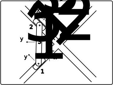
In this project, a rigid bar is connected to two sliding pistons along the diagonal tracks. As the pistons move along the tracks, the rigid bar rotates at a constant rate, $\dot{\theta}_3 = 2~rad/s$. The figure above has three relative coordinate systems that move with the bodies:

1. $x_1-y_1-$ describes piston 1 position and orientation, $\theta_1$
2. $x_2-y_2-$ describes piston 2 position and orientation, $\theta_2$
3. $x_3-y_3-$ describes the rigid bar position and orientation, $\theta_3$

Each of the pistons are on tracks at $\pm 45^o$ and the rotating rigid bar is 10 cm. The hinges are mounted to the center of the pistons connecting the ends of the rigid bar.

In this project, you need to

1. determine constraint equations $C(\mathbf{q},~t)$
2. solve for the velocities, $\dot{q}$ and accelerations, $\ddot{q}$
3. visualize the motion of the system as the rigid bar goes through at least one full rotation

Results

Mechanism Animation (2 Full Rotations)

Kinematic Dashboard

Positions vs. Time

Velocities vs. Time

Accelerations vs. Time

Piston Trajectories

Bar Center Trajectory

Conclusions

Several conclusions can be drawn from the results above. First, the piston trajectories confirm that Piston 1 slides along the $+45^{\circ}$ track and Piston 2 slides along the $-45^{\circ}$ track, as enforced by the prismatic joint constraints. The bar center traces a perfect circle of radius $L/2 = 0.05$ m.

From the position plots, one can observe that $x_1$, $y_1$, $\theta_1$, and $x_2$, $y_2$, $\theta_2$ are consistent with their respective constraint equations. This can also be observed for all generalized parameters in the velocity and acceleration plots, thus confirming that the constraints were implemented correctly and the simulation returned a valid solution. Furthermore, since the bar rotates at a constant rate, the position, velocity, and acceleration plots all exhibit sinusoidal behavior.

The analytical validation printout demonstrates that the numerical solver (using the NonlinearSolve package for positions and the backslash operator for velocities and accelerations) agrees with the analytical solution to within floating-point precision. The constraint residual also remains effectively zero throughout the simulation, verifying that all constraints are satisfied at every time step.

Overall, this project demonstrates the capabilities of using constraint-based methods to solve kinematics problems. By creating constraint equations, computing their Jacobian, and solving for the system's position, velocity, and acceleration at each time step, one can analyze complex problems without deriving explicit equations of motion. Furthermore, this general framework can be extended to systems with more bodies and/or constraints!

Derivations

Note: the following derivations use GitHub-compatible Markdown/LaTeX formatting. Certain expressions (e.g., subscripts or matrix notation) may need modification for standard LaTeX/Markdown environments.

In planar (2D) multibody dynamics, each unconstrained body has 3 degrees of freedom:

• Translation in the $x$-direction
• Translation in the $Y$-direction
• Rotation by angle $\theta$. Therefore, the generalized coordinate vector for this project can be expressed as:

$$ \vec{q} = \begin{bmatrix} x_1 \\ y_1 \\ \theta_1 \\ x_2 \\ y_2 \\ \theta_2 \\ x_3 \\ y_3 \\ \theta_3 \end{bmatrix} $$

If a the center of body i is located at $\vec{R}_i = [x_i, y_i]^T$ in the global coordinate system and orientation $\theta_i$, then point p located at $\vec{s}^{(i)} = [s_x, s_y]^T$ in the body's local frame has global position:

$$ \vec{r}_P = \vec{R}_i + A(\theta_i) , \vec{s}^{(i)} $$

Where $A(\theta_i)$ is the rotation matrix:

$$ A(\theta_i) = \begin{bmatrix} \cos\theta_i & -\sin\theta_i \\ \sin\theta_i & \cos\theta_i \end{bmatrix} $$

For the system above, the hinges are mounted at the center of each piston. So the hinge location in each piston's local frame is at the origin: $\vec{s}_1 = \vec{s}_2 = [0, 0]^T$. Therefore, the hinge for each piston can be expressed in global coordinates as:

$$ \begin{aligned} \vec{r}_{hinge,1} &= \vec{R}_1 + A(\theta_1) , \vec{s}_1 \\ &= \begin{bmatrix} x_1 \\ y_1 \end{bmatrix} \end{aligned} $$ $$ \begin{aligned} \vec{r}_{hinge,2} &= \vec{R}_2 + A(\theta_2) , \vec{s}_2 \\ &= \begin{bmatrix} x_2 \\ y_2 \end{bmatrix} \end{aligned} $$

Now, the rigid bar has length $L$, and its local $x$-axis runs along its length. The center of the bar in global coordinates can be expressed as $\vec{R}_{3} = [x_3, y_3]^T$. End A connects to Piston 1 at local coordinates $\vec{s}_{3A} = \left[-\frac{L}{2}, 0\right]^T$. In global coordinates, this can be expressed as:

$$ \begin{aligned} \vec{r}_A &= \vec{R}_3 + A(\theta_3) , \vec{s}_{3A} \\ &= \begin{bmatrix} x_3 \\ y_3 \end{bmatrix} + \begin{bmatrix} \cos\theta_3 & -\sin\theta_3 \\ \sin\theta_3 & \cos\theta_3 \end{bmatrix} \begin{bmatrix} -\frac{L}{2} \\ 0 \end{bmatrix} \\ &= \begin{bmatrix} x_3 - \frac{L}{2} \cos\theta_3 \\ y_3 - \frac{L}{2} \sin\theta_3 \end{bmatrix} \end{aligned} $$

End B connects to Piston 2 at local coordinates $\vec{s}_{3B} = \left[\frac{L}{2}, 0\right]^T$. In global coordinates, this can be expressed as:

$$ \begin{aligned} \vec{r}_B &= \vec{R}_3 + A(\theta_3) , \vec{s}_{3B} \\ &= \begin{bmatrix} x_3 \\ y_3 \end{bmatrix} + \begin{bmatrix} \cos\theta_3 & -\sin\theta_3 \\ \sin\theta_3 & \cos\theta_3 \end{bmatrix} \begin{bmatrix} \frac{L}{2} \\ 0 \end{bmatrix} \\ &= \begin{bmatrix} x_3 + \frac{L}{2} \cos\theta_3 \\ y_3 + \frac{L}{2} \sin\theta_3 \end{bmatrix} \end{aligned} $$

The constraint equations can now be assembled. A prismatic (sliding) joint constrains Piston 1 to the $+45^\circ$ track. Therefore, the center of Piston 1 is constrained to:

$$ C_1 = y_1 - x_1 = 0 $$

and its orientation is constrained to:

$$ C_2 = \theta_1 - \pi/4 = 0 $$

Similarly, a prismatic (sliding) joint also constrains Piston 2 to the $-45^\circ$ track. Therefore, the center of Piston 2 is constrained to:

$$ C_3 = y_2 + x_2 = 0 $$

and its orientation is constrained to:

$$ C_4 = \theta_2 + \pi/4 = 0 $$

Next, a revolute (hinge) joint connects the center of Piston 1 to end A of the bar. As a result, these two points must have the same global position:

$$ \begin{aligned} \vec{r}_{hinge,1} &= \vec{r}_A \\ \begin{bmatrix} x_1 \\ y_1 \end{bmatrix} &= \begin{bmatrix} x_3 - \frac{L}{2} \cos\theta_3 \\ y_3 - \frac{L}{2} \sin\theta_3 \end{bmatrix} \end{aligned} $$

Which yields the following constraint equations for the x-component:

$$ C_5 = x_1 - x_3 + \frac{L}{2} \cos\theta_3 = 0 $$

and the y-component:

$$ C_6 = y_1 - y_3 + \frac{L}{2} \sin\theta_3 = 0 $$

A revolute (hinge) joint also connects the center of Piston 2 to end B of the bar:

$$ \begin{aligned} \vec{r}_{hinge,2} &= \vec{r}_B \\ \begin{bmatrix} x_2 \\ y_2 \end{bmatrix} &= \begin{bmatrix} x_3 + \frac{L}{2} \cos\theta_3 \\ y_3 + \frac{L}{2} \sin\theta_3 \end{bmatrix} \end{aligned} $$

Which yields the following constraint equations for the x-component:

$$ C_7 = x_2 - x_3 - \frac{L}{2} \cos\theta_3 = 0 $$

and the y-component:

$$ C_8 = y_2 - y_3 - \frac{L}{2} \sin\theta_3 = 0 $$

Finally, the bar rotates at a constant rate of $\dot{\theta}_3 = \omega = 2$ rad/s. Integrating this with $\theta_3(0) = 0$ yields:

$$ C_9 = \theta_3 - \omega t = 0 $$

Therefore, the full constraint vector can be written as:

$$ \vec{C}(\vec{q}, t) = \begin{bmatrix} C_1 \\ C_2 \\ C_3 \\ C_4 \\ C_5 \\ C_6 \\ C_7 \\ C_8 \\ C_9 \end{bmatrix} = \begin{bmatrix} y_1 - x_1 \\ \theta_1 - \pi/4 \\ y_2 + x_2 \\ \theta_2 + \pi/4 \\ x_1 - x_3 + \frac{L}{2} \cos\theta_3 \\ y_1 - y_3 + \frac{L}{2} \sin\theta_3 \\ x_2 - x_3 - \frac{L}{2} \cos\theta_3 \\ y_2 - y_3 - \frac{L}{2} \sin\theta_3 \\ \theta_3 - \omega t \end{bmatrix} = \vec{0} $$

The constraint Jacobian, $C_q = \frac{\partial \vec{C}}{\partial \vec{q}}$ can now be evaluated as:

$$ C_q = \begin{bmatrix} -1 & 1 & 0 & 0 & 0 & 0 & 0 & 0 & 0 \\ 0 & 0 & 1 & 0 & 0 & 0 & 0 & 0 & 0 \\ 0 & 0 & 0 & 1 & 1 & 0 & 0 & 0 & 0 \\ 0 & 0 & 0 & 0 & 0 & 1 & 0 & 0 & 0 \\ 1 & 0 & 0 & 0 & 0 & 0 & -1 & 0 & -\frac{L}{2}\sin\theta_3 \\ 0 & 1 & 0 & 0 & 0 & 0 & 0 & -1 & \frac{L}{2}\cos\theta_3 \\ 0 & 0 & 0 & 1 & 0 & 0 & -1 & 0 & \frac{L}{2}\sin\theta_3 \\ 0 & 0 & 0 & 0 & 1 & 0 & 0 & -1 & -\frac{L}{2}\cos\theta_3 \\ 0 & 0 & 0 & 0 & 0 & 0 & 0 & 0 & 1 \end{bmatrix} $$

the partial time derivative vector, $\vec{C}_t = \frac{\partial \vec C}{\partial t}$ can be evaluated as

$$ \vec{C}_t = \begin{bmatrix} 0 \\ 0 \\ 0 \\ 0 \\ 0 \\ 0 \\ 0 \\ 0 \\ -\omega \end{bmatrix} $$

Thus, the velocity constraint equation $C_q , \dot{\vec{q}} = - \vec{C}_t$ can be constructed:

$$ \begin{bmatrix} -1 & 1 & 0 & 0 & 0 & 0 & 0 & 0 & 0 \\ 0 & 0 & 1 & 0 & 0 & 0 & 0 & 0 & 0 \\ 0 & 0 & 0 & 1 & 1 & 0 & 0 & 0 & 0 \\ 0 & 0 & 0 & 0 & 0 & 1 & 0 & 0 & 0 \\ 1 & 0 & 0 & 0 & 0 & 0 & -1 & 0 & -\frac{L}{2}\sin\theta_3 \\ 0 & 1 & 0 & 0 & 0 & 0 & 0 & -1 & \frac{L}{2}\cos\theta_3 \\ 0 & 0 & 0 & 1 & 0 & 0 & -1 & 0 & \frac{L}{2}\sin\theta_3 \\ 0 & 0 & 0 & 0 & 1 & 0 & 0 & -1 & -\frac{L}{2}\cos\theta_3 \\ 0 & 0 & 0 & 0 & 0 & 0 & 0 & 0 & 1 \end{bmatrix} \begin{bmatrix} \dot{x}_1 \\ \dot{y}_1 \\ \dot{\theta}_1 \\ \dot{x}_2 \\ \dot{y}_2 \\ \dot{\theta}_2 \\ \dot{x}_3 \\ \dot{y}_3 \\ \dot{\theta}_3 \\ \end{bmatrix} = \begin{bmatrix} 0 \\ 0 \\ 0 \\ 0 \\ 0 \\ 0 \\ 0 \\ 0 \\ \omega \end{bmatrix} $$

The acceleration constraint equation can be found by taking the time derivative of the velocity equation:

$$ \frac{d}{dt} \left(C_q , \dot{\vec{q}}\right) + \frac{d}{dt}\left(\vec{C}_t\right) = \vec{0} $$

The equation above can be rewritten as:

$$ C_q , \ddot{\vec{q}} = \vec{\gamma} $$

where:

$$ \vec{\gamma} = -\frac{d C_q}{dt} , \dot{\vec{q}} - \frac{d \vec{C}_t}{dt} $$

Since $\theta_3$ changes with time, $\frac{d}{dt} f\left(\theta_3\right) = \frac{d f}{d \theta_3} \dot{\theta}_3$. So:

$$ \frac{d C_q}{d t} = \begin{bmatrix} 0 & 0 & 0 & 0 & 0 & 0 & 0 & 0 & 0 \\ 0 & 0 & 0 & 0 & 0 & 0 & 0 & 0 & 0 \\ 0 & 0 & 0 & 0 & 0 & 0 & 0 & 0 & 0 \\ 0 & 0 & 0 & 0 & 0 & 0 & 0 & 0 & 0 \\ 0 & 0 & 0 & 0 & 0 & 0 & 0 & 0 & \left(-\frac{L}{2}\cos\theta_3\right)\dot{\theta}_3 \\ 0 & 0 & 0 & 0 & 0 & 0 & 0 & 0 & \left(-\frac{L}{2}\sin\theta_3\right)\dot{\theta}_3 \\ 0 & 0 & 0 & 0 & 0 & 0 & 0 & 0 & \left(\frac{L}{2}\cos\theta_3\right)\dot{\theta}_3 \\ 0 & 0 & 0 & 0 & 0 & 0 & 0 & 0 & \left(\frac{L}{2}\sin\theta_3\right)\dot{\theta}_3 \\ 0 & 0 & 0 & 0 & 0 & 0 & 0 & 0 & 0 \end{bmatrix} $$

and:

$$ \frac{d C_q}{dt} , \dot{\vec{q}} = \begin{bmatrix} 0 \\ 0 \\ 0 \\ 0 \\ \left(-\frac{L}{2}\cos\theta_3\right)\dot{\theta}_3^2 \\ \left(-\frac{L}{2}\sin\theta_3\right)\dot{\theta}_3^2 \\ \left(\frac{L}{2}\cos\theta_3\right)\dot{\theta}_3^2 \\ \left(\frac{L}{2}\sin\theta_3\right)\dot{\theta}_3^2 \\ 0 \end{bmatrix} $$

Since $\frac{d C_t}{d t} = \vec{0}$:

$$ \vec{\gamma} = \begin{bmatrix} 0 \\ 0 \\ 0 \\ 0 \\ \left(\frac{L}{2}\cos\theta_3\right)\dot{\theta}_3^2 \\ \left(\frac{L}{2}\sin\theta_3\right)\dot{\theta}_3^2 \\ \left(-\frac{L}{2}\cos\theta_3\right)\dot{\theta}_3^2 \\ \left(-\frac{L}{2}\sin\theta_3\right)\dot{\theta}_3^2 \\ 0 \end{bmatrix} $$

and the final acceleration constraint equation can be constructed:

$$ \begin{bmatrix} -1 & 1 & 0 & 0 & 0 & 0 & 0 & 0 & 0 \\ 0 & 0 & 1 & 0 & 0 & 0 & 0 & 0 & 0 \\ 0 & 0 & 0 & 1 & 1 & 0 & 0 & 0 & 0 \\ 0 & 0 & 0 & 0 & 0 & 1 & 0 & 0 & 0 \\ 1 & 0 & 0 & 0 & 0 & 0 & -1 & 0 & -\frac{L}{2}\sin\theta_3 \\ 0 & 1 & 0 & 0 & 0 & 0 & 0 & -1 & \frac{L}{2}\cos\theta_3 \\ 0 & 0 & 0 & 1 & 0 & 0 & -1 & 0 & \frac{L}{2}\sin\theta_3 \\ 0 & 0 & 0 & 0 & 1 & 0 & 0 & -1 & -\frac{L}{2}\cos\theta_3 \\ 0 & 0 & 0 & 0 & 0 & 0 & 0 & 0 & 1 \end{bmatrix} \begin{bmatrix} \ddot{x}_1 \\ \ddot{y}_1 \\ \ddot{\theta}_1 \\ \ddot{x}_2 \\ \ddot{y}_2 \\ \ddot{\theta}_2 \\ \ddot{x}_3 \\ \ddot{y}_3 \\ \ddot{\theta}_3 \\ \end{bmatrix} = \begin{bmatrix} 0 \\ 0 \\ 0 \\ 0 \\ \left(\frac{L}{2}\cos\theta_3\right)\dot{\theta}_3^2 \\ \left(\frac{L}{2}\sin\theta_3\right)\dot{\theta}_3^2 \\ \left(-\frac{L}{2}\cos\theta_3\right)\dot{\theta}_3^2 \\ \left(-\frac{L}{2}\sin\theta_3\right)\dot{\theta}_3^2 \\ 0 \end{bmatrix} $$

The solution process for the system above will consist of 3 sequential steps at each time step $t_i$:

Step 01: Solve for Positions (Nonlinear)

• Find $\vec{q}$ such that $\vec{C}\left(\vec{q}, t\right) = \vec{0}$ using a nonlinear iterative solver and the solution from the previous step as an initial guess.

Step 02: Solve for Velocities (Linear)

• Solve $C_q , \dot{\vec{q}} = -\vec{C}_t$ for $\dot{\vec{q}}$ using positions found in Step 01.

Step 03: Solve for Accelerations (Linear)

• Solve $C_q , \ddot{\vec{q}} = \vec{\gamma}$ for $\ddot{\vec{q}}$ using both positions found in Step 01 and velocities found in Step 02.

The coordinates of the system above can also be solved for analytically. The analytical solution can be used as an initial guess for the numerical solver, and also as a benchmark to verify the numerical results. From constraint equations $C_5$ and $C_6$:

$$ x_1 = x_3 - \frac{L}{2} \cos\theta_3 \qquad (C_5) $$ $$ y_1 = y_3 - \frac{L}{2} \sin\theta_3 \qquad (C_6) $$

Substituting $C_5$ and $C_6$ into $C_1 = y_1 - x_1 = 0$:

$$ \left(y_3 - \frac{L}{2} \sin\theta_3\right) - \left(x_3 - \frac{L}{2} \cos\theta_3\right) = 0 $$ $$ y_3 - x_3 = \frac{L}{2}\left(\sin\theta_3 - \cos\theta_3\right) \qquad (a) $$

From constraint equations $C_7$ and $C_8$:

$$ x_2 = x_3 + \frac{L}{2} \cos\theta_3 \qquad (C_7) $$ $$ y_2 = y_3 + \frac{L}{2} \sin\theta_3 \qquad (C_8) $$

Substituting $C_7$ and $C_8$ into $C_3 = y_2 + x_2 = 0$:

$$ \left(y_3 + \frac{L}{2} \sin\theta_3 \right) + \left(x_3 + \frac{L}{2} \cos\theta_3\right) = 0 $$ $$ y_3 + x_3 = -\frac{L}{2}\left(\sin\theta_3 + \cos\theta_3\right) \qquad (b) $$

Therefore, the system has been reduced to two equations and two unknowns. Adding equations $a$ and $b$:

$$ (y_3 - x_3) + (y_3 + x_3) = \frac{L}{2}\left(\sin\theta_3 - \cos\theta_3\right) - \frac{L}{2}\left(\sin\theta_3 + \cos\theta_3\right) $$ $$ 2 y_3 = -\frac{L}{2} (2 \cos\theta_3) $$ $$ y_3 = -\frac{L}{2} \cos\theta_3 $$

Subtracting equation $a$ from $b$:

$$ (y_3 + x_3) - (y_3 - x_3) = -\frac{L}{2}\left(\sin\theta_3 + \cos\theta_3\right) - \frac{L}{2}\left(\sin\theta_3 - \cos\theta_3\right) $$ $$ 2x_3 = -\frac{L}{2}(2\sin(\theta_3)) $$ $$ x_3 = -\frac{L}{2}\sin\theta_3 $$

To find the piston positions, $y_3$ and $x_3$ can be substituted back into constraint equations $C_5$, $C_6$, $C_7$, and $C_8$:

$$ x_1 = -\frac{L}{2}\sin\theta_3 - \frac{L}{2} \cos\theta_3 = -\frac{L}{2}\left(\sin\theta_3 + \cos\theta_3\right) $$ $$ y_1 = -\frac{L}{2} \cos\theta_3 - \frac{L}{2} \sin\theta_3 = -\frac{L}{2}\left(\cos\theta_3 + \sin\theta_3 \right) = x_1 $$ $$ x_2 = -\frac{L}{2}\sin\theta_3 + \frac{L}{2} \cos\theta_3 = \frac{L}{2} \left(\cos\theta_3 - \sin\theta_3 \right) $$ $$ y_2 = -\frac{L}{2} \cos\theta_3 + \frac{L}{2} \sin\theta_3 = \frac{L}{2} \left(\sin\theta_3 - \cos\theta_3 \right) = -x_2 $$

To find the analytical velocities, each position above can be differentiated with respect to time:

$$ \dot{x}_1 = \frac{L}{2}\left(\sin\theta_3 - \cos\theta_3\right)\omega $$ $$ \dot{y}_1 = \dot{x}_1 = \frac{L}{2}\left(\sin\theta_3 - \cos\theta_3\right)\omega $$ $$ \dot{x}_2 = -\frac{L}{2}\left(\sin\theta_3 + \cos\theta_3 \right)\omega $$ $$ \dot{y}_2 = -\dot{x}_2 = \frac{L}{2}\left(\sin\theta_3 + \cos\theta_3 \right)\omega $$ $$ \dot{x}_3 = -\frac{L}{2} \cos\theta_3 \omega $$ $$ \dot{y}_3 = \frac{L}{2} \sin\theta_3 \omega $$ $$ \dot{\theta}_1 = 0 $$ $$ \dot{\theta}_2 = 0 $$ $$ \dot{\theta}_3 = \omega $$

To find the analytical accelerations, each velocity above can be differentiated with respect to time:

$$ \ddot{x}_1 = \frac{L}{2} \left(\cos\theta_3 + \sin\theta_3 \right)\omega^2 $$ $$ \ddot{y}_1 = \ddot{x}_1 = \frac{L}{2} \left(\cos\theta_3 + \sin\theta_3 \right)\omega^2 $$ $$ \ddot{x}_2 = \frac{L}{2} \left(\sin\theta_3 - \cos\theta_3 \right)\omega^2 $$ $$ \ddot{y}_2 = -\ddot{x}_2 = -\frac{L}{2} \left(\sin\theta_3 - \cos\theta_3 \right)\omega^2 $$ $$ \ddot{x}_3 = \frac{L}{2} \sin\theta_3 \omega^2 $$ $$ \ddot{y}_3 = \frac{L}{2} \cos\theta_3 \omega^2 $$ $$ \ddot{\theta}_1 = 0 $$ $$ \ddot{\theta}_2 = 0 $$ $$ \ddot{\theta}_3 = 0 $$

This confirms that the bar center traces a circle of radius $L/2$ and the pistons oscillate along their tracks.

Reproducing Results

From the project directory, run:

julia main.jl 

The program may take a few minutes to run. All final plots are output to the results/ directory.

Project Dependencies

This project was developed and tested with Julia version 1.12.4

The following packages are required:

• NonlinearSolve
• LinearAlgebra
• Plots
• Measures
• LaTeXStrings

Project Structure

project_02-15/
|
├───── archive/ # old plots and files
|
├───── notes/   # hand calculations
|
├───── results/ # program outputs (plots)
|
├───── src/     # source Code
|       |
|       ├───── constraints.jl      # constraint equations and analytical solutions
|       |
|       ├───── kinematics.jl       # position, velocity, and acceleration solvers
|       |
|       └───── visualize.jl        # plotting and animation functions
|
├───── main.jl                     # main driver
|
└───── README.md                   # project documentation