
Raptor is a Python-based simulation tool for estimating porosity-related defects in Laser Powder Bed Fusion (LPBF) additive manufacturing processes. It uses a computationally efficient geometric approach to model the dynamic melt pool and identify regions of unmelted material, which correspond to lack-of-fusion pores. The core of Raptor is a geometric model of the melt pool cross-section whose dimensions (width, depth, and height) oscillate over time. By analyzing the volume swept by this dynamic melt pool along the laser scan paths, Raptor generates a 3D map of the final part's porosity.
This project is licensed under the BSD 3-Clause License.
- Vamsi Subraveti, Vanderbilt University, vamsi.r.subraveti@vanderbilt.edu
- John Coleman, Oak Ridge National Laboratory, colemanjs@ornl.gov
- Çağlar Oskay, Vanderbilt University, caglar.oskay@vanderbilt.edu
- Alex Plotkowski, Oak Ridge National Laboratory, plotkowskiaj@ornl.gov
Raptor predicts porosity by following a multi-step process:
- Domain Voxelization: A 3D bounding box, or Representative Volume Element (RVE), is defined and discretized into a uniform grid of voxels.
- Scan Path Ingestion: Scan path data is used to calculate the timing and trajectory for each laser vector.
- Dynamic Melt Pool Definition: For each melt pool dimension (width, depth, height), the input time-series data is converted into a Fourier series (a sum of cosine functions). This creates a dynamic, time-dependent model of the melt pool's cross-sectional shape, which is modeled using modified Lamé curves. To capture stochastic process variations, a random phase shift can be applied to the Fourier series for each scan vector.
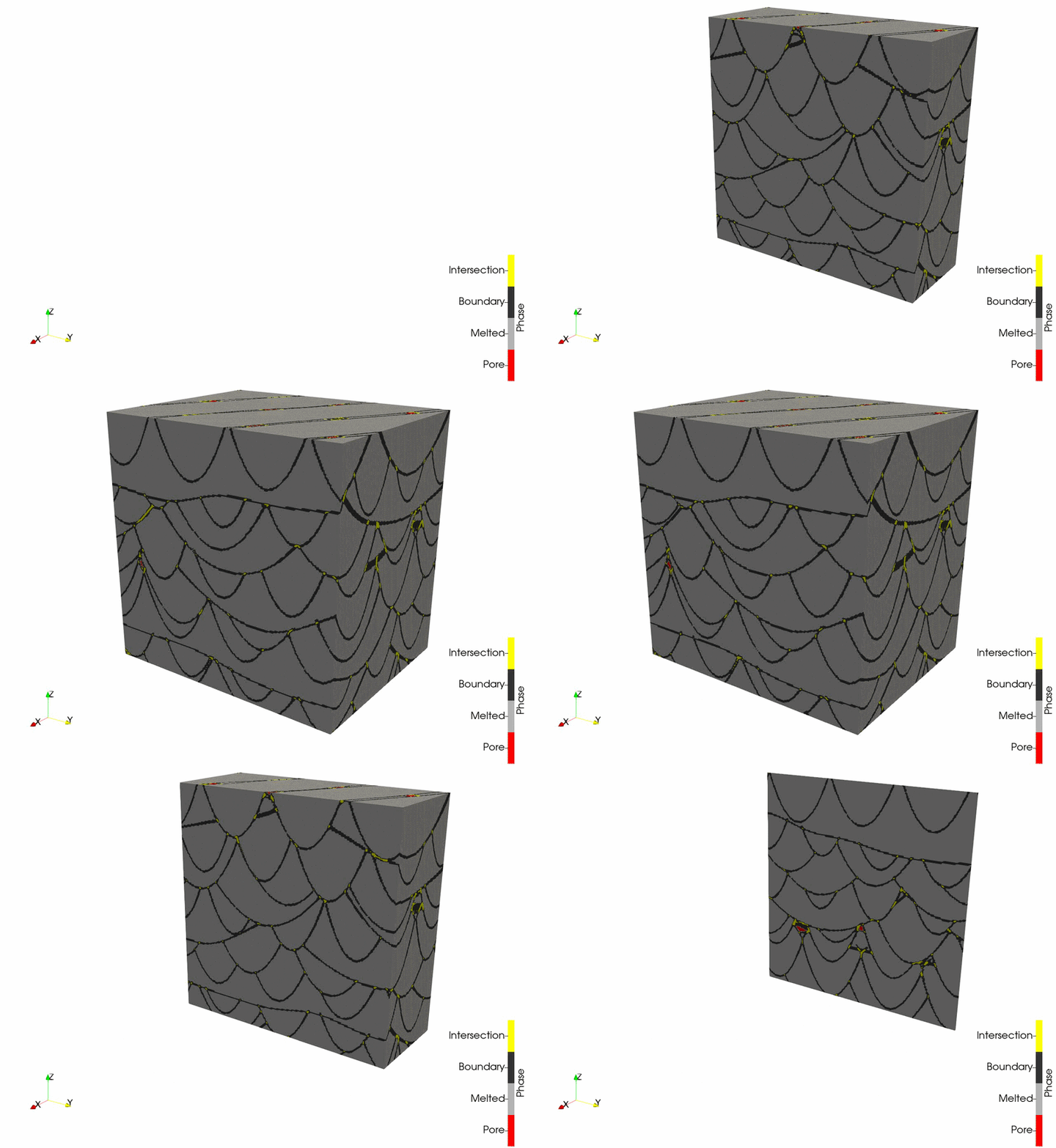
- Melt Mask Calculation: The core of the simulation iterates through each voxel in the domain. For each scan vector that passes near the voxel, it calculates the instantaneous melt pool shape and determines the voxel state. The voxel is either unmelted (0), in the interior of the melt pool (1), on the boundary of the melt pool (2), or at an intersection of melt pool boundaries (3). The voxel state updates dynamically as successive scan vectors melt it or interact with it along a melt pool boundary. The outcome of this process is a simulated volume of overlapping melt pools, flagging melted voxels, boundary voxels, intersection voxels, and voxels that make up the defect structure. The core geometry computations are executed with a high-performance parallel kernel, just-in-time (JIT) compiled with Numba. This enables the rapid analysis of large, industrially relevant domains.
- Porosity Prediction: Any voxel that is not melted by the end of the simulation is flagged as porosity.
- Boundary Tracking: Voxels that are close to local melt pool boundaries are flagged as boundaries.
- Intersection Tracking: Voxels that are incident with two or more boundaries are flagged as intersection points.
- Analysis and Output: The final 3D volume is saved in the binary VTK ImageData (
.vti) format. The morphological characteristics (e.g., volume, surface area, equivalent diameter) of contiguous pore structures can be quantified using thescikit-imagelibrary and saved to a.csvfile.
Raptor requires Python 3.10 or newer. The following Python packages are necessary:
    numpy, numba, psutil, scipy, matplotlib, PyYAML, vtk,
scikit-image, pandas, pyvista- NumPy: For numerical operations and array manipulation.
- Numba: For JIT compilation and performance acceleration.
- psutil: For detecting available process and system memory.
- SciPy: For signal filtering and statistical calculations.
- Matplotlib: For optional melt pool signal plots.
- PyYAML: For reading and parsing YAML configuration files.
- VTK: For writing the output porosity map in
.vtiformat. - scikit-image: For calculating pore morphologies.
- pandas: For writing morphology information to
.csv. - pyvista: For visualization of
.vtiresults.
From the cloned Raptor directory, create an isolated environment, install the package, configure a persistent cache inside the repository, and warm the production Numba signatures:
python -m venv .venv
source .venv/bin/activate
python -m pip install --upgrade pip
python -m pip install .

export NUMBA_CACHE_DIR="$(pwd)/.numba-cache"
raptor-warm-cache --cache-dir "$NUMBA_CACHE_DIR"
Keep the virtual environment active and NUMBA_CACHE_DIR set when running
Raptor. In a new shell, run source .venv/bin/activate and repeat the
export command. Cache warming is optional; without it, the first simulation
compiles and caches the kernels automatically. Use a separate cache directory
for each Python/Numba version and CPU architecture.
The project is organized into several modules:
cli.py: Handles command-line argument parsing and manages the main simulation workflow.api.py: Provides high-level functions for creating the grid, melt pool, running the simulation, and writing output files.core.py: Contains melt geometry and the Numba-accelerated voxel kernel.spatial.py: Builds exact, ordered spatial candidates for path vectors.spectral.py: Plans and evaluates accuracy-controlled melt-pool histories.resources.py: Resolves memory budgets and spectral-table batching.morphology.py: Counts phases and labels sparse defects.structures.py: Defines the main data structures for the simulation (Grid,MeltPool,PathVector).io.py: Contains functions for reading and parsing input files (scan paths, melt pool data).utilities.py: Includes helper classes, such as theScanPathBuilderfor generating scan strategies.
Raptor can be used in two primary ways: through its Command-Line Interface (CLI) for quick, configuration-driven simulations, or as a Python Library (API) for integration into custom scripts and simulation workflows.
The CLI usage requires scan path files corresponding to build information. These scan path files can be generated with the ScanPathBuilder class in raptor.utilities. The CLI is controlled by a single YAML input file that defines all inputs, parameters, and outputs. The CLI example contains a single scan path to show functionality and observe the fluctuations of the simulated melt pool. The API example is recommended for a more descriptive simulation of undermelting-induced defects.
How to Run (CLI):
- Prepare Inputs: Create scan path files, melt pool data files, and an
input.yamlfile (detailed below). - Execute Script: Run the following command from your terminal, providing the path to your configuration file:
raptor path/to/your/input.yaml
- Check Outputs:
- Progress will be printed to the console.
- The 3D porosity map is saved to the
.vtifile specified in the config. - The pore morphology data is saved to the
.csvfile if configured. The example does not save morphology information.
Running Raptor from the CLI requires a YAML input file to specify all parameters.
Example input.yaml:
# List of scan path files (relative to this config file's location)
scan_paths:
  - "scan_paths/layer_01.txt"
  - "scan_paths/layer_02.txt"

parameters:
  layer_height: 5.0e-5      # Layer height in meters
  voxel_resolution: 5.0e-6  # Voxel resolution in meters
  enable_random_segment_phase: true # Use random phases for melt pool oscillations per vector
  random_seed: 42
  tile_width: null
  spectral_error_fraction: 0.25
  memory_limit_mb: null

# Melt pool dimension data. Must be 'time_series' (time, value) data.
melt_pool_data:
  width:
    type: "time_series"
    file_name: "melt_pool_data/width_timeseries.txt"
    nmodes: 10          # Number of Fourier modes to extract
    scale: 1.0          # Multiplicative scaling factor for amplitudes
  depth:
    type: "time_series"
    file_name: "melt_pool_data/depth_timeseries.txt"
    nmodes: 10
    scale: 1.0
    shape: 2.0          # Shape factor 'n' for the Lamé curve (n=2 is elliptical)
  height:
    type: "time_series"
    file_name: "melt_pool_data/height_timeseries.txt"
    nmodes: 10
    scale: 1.0
    shape: 0.5          # n=0.5 is bell-shaped

# Representative Volume Element (RVE) defining the simulation domain
rve:
  min_point: [0.0, 0.0, 0.0]          # [x, y, z] minimum corner in meters
  max_point: [0.001, 0.001, 0.0001]   # [x, y, z] maximum corner in meters

# Output settings
output:
  vtk:
    file_name: "porosity_map.vti"
  morphology:
    file_name: "morphology.csv"
    # Properties from scikit-image regionprops
    # See: https://scikit-image.org/docs/stable/api/skimage.measure.html#skimage.measure.regionprops
    fields:
      - "label"
      - "area"
      - "equivalent_diameter_area"
The optional CLI controls correspond to the compute_porosity keyword
arguments described below. If memory_limit_mb is null, Raptor checks the
RAPTOR_MEMORY_LIMIT_MB environment variable and otherwise uses 80% of
currently available memory.
-
Scan Path Files: Each file in
scan_pathsshould be a space-delimited text file. The first line is treated as a header and is skipped. Format per line:mode x y z power parametermode: Integer (0for line raster,1for point source/delay).x, y, z: Float endpoint coordinates in meters.power: Float laser power in Watts (for information, not used in the geometry model).parameter: Float (mode=0: scanning speed in m/s;mode=1: duration in seconds).
Example
layer_01.txt:# Mode X_end(m) Y_end(m) Z_end(m) Power(W) Speed(m/s)_or_Time(s) 1 0.000 0.000 0.000 0 0.00001 0 0.001 0.000 0.000 200 0.8 0 0.001 0.0001 0.000 200 0.8- The RVE min and max points filter the scan paths for those that are near the box defined by
min_pointandmax_point; a large number of scan path files (such as from a part-scale build) can be downselected using this parameter setting.
-
Melt Pool Data Files: These files provide the data for the
melt_pool_datasection of the config.- With
type: "time_series", the file should be a two-column text or CSV file:[time, value].
- With
The API supports programmatic parameter studies, custom workflows, and
integration with other tools. The example in examples/api_example/rve.py
simulates defects in a cube with a 500 µm edge length.
The following is a breakdown of the main steps for running a simulation programmatically.
First, define the simulation domain (RVE) by specifying its minimum and maximum coordinates and the desired voxel resolution. The create_grid function then generates the grid object.
import numpy as np
from raptor.api import create_grid

# 1. Create voxel grid for the representative volume element (RVE)
min_point = np.array([0.0, 0.0, 0.0])
max_point = np.array([5.0e-4, 5.0e-4, 5.0e-4])
bound_box = np.array([min_point, max_point])
voxel_resolution = 5.0e-6

grid = create_grid(voxel_resolution, bound_box=bound_box)Use the ScanPathBuilder utility to programmatically generate a scan strategy. This builder takes process parameters like power, speed, and hatch spacing to create a list of PathVector objects for the simulation.
from raptor.utilities import ScanPathBuilder

# 2. Create path vectors through the representative volume element (RVE)
power = 370
velocity = 1.7
hatch_spacing = 140e-6
layer_height = 30e-6
rotation = 67
scan_extension = max(max_point - min_point)
extra_layers = 0

scan_path_builder = ScanPathBuilder(
    bound_box,
    power,
    velocity,
    hatch_spacing,
    layer_height,
    rotation,
    scan_extension,
    extra_layers,
)

scan_path_builder.generate_layers()
path_vectors = scan_path_builder.process_vectors()Load the melt pool dimension data (in this case, from a text file) and use
create_melt_pool to construct the MeltPool object. The API allows you to
set a scaling factor for each dimension and shape factors for the vertical
dimensions. The transverse width exponent is fixed at two.
from pathlib import Path
from raptor.io import read_data
from raptor.api import create_melt_pool

# 3. Create melt pools given a width sequence
SCRIPT_DIR = Path(__file__).resolve().parent
melt_pool_data_path = (
    SCRIPT_DIR / ".." / "data" / "meltPoolData" / "ULI_v1700_theta0_widths.txt"
)
width_data = read_data(melt_pool_data_path)
n_modes = 50

# scale melt pool data by constant factor
width_scale = 1.0
depth_scale = 0.8
height_scale = 0.4

# The transverse exponent is fixed at two. Select the vertical exponents
# (1 = parabola, 2 = ellipse).
width_shape = 2
height_shape = 1
depth_shape = 1

melt_pool_dict = {
    "width": (width_data, n_modes, width_scale, width_shape),
    "depth": (width_data, n_modes, depth_scale, depth_shape),
    "height": (width_data, n_modes, height_scale, height_shape),
}

melt_pool = create_melt_pool(melt_pool_dict, enable_random_phases=False)With the grid, path vectors, and melt pool defined, call the main compute_porosity function. This runs the core Numba-accelerated simulation and returns the final 3D porosity field as a NumPy array.
from raptor.api import compute_porosity

# 4. Compute porosity using melt pool mask
porosity = compute_porosity(
    grid,
    path_vectors,
    melt_pool,
    random_seed=42,
    tile_width=None,
    spectral_error_fraction=0.25,
    memory_limit_mb=None,
)
The optional controls have the following behavior:
random_seedmakes randomly generated segment phases reproducible.tile_width=Noneselects the automatic spatial-index tile width.spectral_error_fraction=0.25limits spectral and interpolation error to one quarter of a voxel.memory_limit_mb=NonechecksRAPTOR_MEMORY_LIMIT_MBand otherwise uses 80% of currently available process memory. An explicit value is a shared per-process budget; it is not divided by the Numba thread count.
When the full spectral table fits, Raptor uses resident execution. Under a smaller memory budget, it streams ordered vector batches without changing the spectral sampling or requested accuracy.
Use the write_vtk helper function to save the resulting porosity NumPy array
to a .vti file for visualization in tools like ParaView. The Phase array
uses 0 for unmelted pore voxels, 1 for melted interior voxels, 2 for melt
pool boundary voxels, and 3 for boundary intersections. ParaView can isolate
the defects within the RVE by thresholding the Phase array around 0.
from raptor.api import write_vtk

# 5. Write porosity field to .VTI
write_vtk(grid.origin, grid.resolution, porosity, "rve.vti")Optionally use compute_morphology and write_morphology to compute
per-defect descriptors such as volume and equivalent diameter. For a full list
of possible descriptors, see the
scikit-image region properties documentation.
from raptor.api import compute_morphology, write_morphology

# 6. Compute morphology
morphology = compute_morphology(porosity, voxel_resolution, ['area', 'equivalent_diameter_area'])
write_morphology(morphology, "rve_morphology.csv")Optionally use visualize to open an interactive PyVista window in the native
coordinate system, measured in meters. The function displays the complete
phase field and, when phase 0 is present, automatically isolates the unmelted
pore voxels in a second view.
from raptor.api import visualize

# 7. Visualize using PyVista
visualize("./rve.vti")
To visualize the example output, uncomment the visualize("./rve.vti") line.
The melt pool measurements in the examples are scans performed in Ti6Al4V from the following study:
- Miner, Justin; Narra, Sneha Prabha (2024). Dataset of Melt Pool Variability Measurements for Powder Bed Fusion - Laser Beam of Ti-6Al-4V. Carnegie Mellon University. Dataset. https://doi.org/10.1184/R1/25696293.v1