R-package which allows users to run multi co-moment structural equation models.
Welcome to the new and improved MCMSEM. If you want to use the MCMSEM version as it was used in the original publication, please go to the v0.1.1 release.
This version is considerably more powerful than our previous version. Some highlights:
- Expanded to allow for any N variables instead of just two (use at your own risk)
- Far more flexibility for custom model creation via MCMSEM model objects
- More detailed fit statistics through custom MCMSEM result objects
- Significantly improved performance, and enabled optimization on GPU
- Asymptotic calculation of standard errors (bootstrapping no longer required)
- Exportable data, making it easier for researchers to share moment matrices for MCMSEM without sharing raw data
- A stationary dynamic VAR(1) kernel alongside the original contemporaneous structural kernel
If you are new to this version of MCMSEM we highly recommend reading our Wiki before starting, as the syntax for using MCMSEM has changed significantly since v0.1.1.
MCMSEM now makes the scientific assumptions about whether to consider, or include, time in the model as a variable explicit:
# Existing behavior and the default
contemporaneous_model <- MCMmodel(ds, kernel = "contemporaneous")

# Stationary observed-state VAR(1)
dynamic_model <- MCMmodel(ds, kernel = "dynamic")
kernel = "static" is a supported, silent alias for "contemporaneous".
Legacy summary and model objects without kernel metadata are also treated as
contemporaneous. The two kernels let the user specify slighlty different types of models and help answer different slightly questions.
Why would we care about this kind of nuance? We (the developers) envision people will use MCMSEM alongside other estimation methods, as the assumptions about moments are novel to many users and people would want some external validaiton. One of the methods we could see people using MCMSEM alongside in psychology would be (random intercept) cross lagged panel models, across 3+ waves of data. Those models define "causal" paths from variabe y on x across time, where y at t-1 influences x at t, as in MCMSEM you'd model the distubances as non-guasian, we'd need a way to model the disturbance of y at t, which hasn't influences x contemoreneously at t yet. This means that to get the same estimate/estimnd out of MCMSEM as you'd get out of a stationary (RI)CLPM, you have to model explict disturbances at each time point t. This requires the new "dynamic" kernel.
Which kernel you pick, essentially the choice you make with respect to how to model the data, depends on whether u conceive as the causal process as a static process that has unfoldeded over the past. For example a static process could be conceived of as follows:
taller adults are heavier, because hte volum of their bodies, all else being equal, is higher, and at similar density this means they are heavier, the process of growth is completed in adults, so there is no dynamic change in height, that results in changes in weight.
An example of a dynamic process can be found in markets (econ) or emotions (psychology), for example:
if I dont sleep well tonight (day = t-2), il be tired tomorrow (day = t), if I then do sleep well (day = t), ill not be tired the day after tomorrow (day = t).
MCMSEM an now model cross sectional data as if its a part of a dynamic system (under assumtions like stationaiity, and non-gaussian disturbances, and all confounders being gausian.).
Contemporaneous structural MCMSEM assumes that the measured variables can be represented by a set of structural equations at one conceptual occasion, such as
The contemporaneous kernel uses the existing Reticular Action Model (RAM) specification. Here,
and
The factor
Stationary dynamic MCMSEM assumes instead that the world evolves through repeated, time-homogeneous transitions,
In the dynamic kernel, the matrix
Consequently, the stationary cumulant of order
In particular,
The parameters in
Alternatively, residual_family = "common_gamma" adds one non-Gaussian
confounder to the stationary marginal state. Write
The loadings may be signed and shape_Gamma is positive. This factor replaces,
rather than supplements, the Gaussian residual in the current API. It is an
additive marginal confounder: it is not an innovation repeatedly propagated
through
gamma_model <- MCMmodel(
  ds, kernel = "dynamic", residual_family = "common_gamma"
)
gamma_parameters <- MCMparameters(gamma_model)
gamma_parameters[grepl("Gamma", gamma_parameters$name), ]MCMparameter() adds auxiliary parameters or converts an existing matrix label. This can help users define parameteric constraints consitent with specific distributions (a gamma distribution for example). Only free parameters are optimized; fixed and derived parameters do not consume degrees of freedom. This signed-gamma constraint uses one positive shape per innovation instead of separate skewness and excess-kurtosis parameters:
model <- MCMmodel(ds, kernel = "dynamic")
model <- MCMparameter(
  model, "shape_Earnings", "free", start = 4, transform = "positive"
)
model <- MCMparameter(
  model, "sign_Earnings", "fixed", value = -1
)
model <- MCMparameter(
  model, "tau_Earnings", "derived",
  expression = ~ sign_Earnings * 2 / sqrt(shape_Earnings)
)
model <- MCMparameter(
  model, "kappa_Earnings", "derived",
  expression = ~ 6 / shape_Earnings
)

MCMparameters(model)
MCMdegreesoffreedom(model)
Expressions use a small validated language rather than arbitrary R evaluation. Supported operations are +, -, *, /, ^, sqrt(), exp(), log(), softplus(), and logistic(). Free starts and fitted estimates are reported on their natural scale; positive and bounded parameters use unconstrained internal optimizer coordinates. Summaries report each parameter's type and expression, derived SEs use the delta method, and fixed SEs are zero when covariance is available.
The same API works for contemporaneous models. There, diagonal K entries are raw standardized fourth moments, so the signed-gamma expression is
~ 3 + 6 / shape; dynamic Kappa entries are fourth cumulants and use
~ 6 / shape.
The current dynamic release supports observed states with at least two variables, a VAR(1) transition, fixed unit innovation variances, diagonal innovation third and fourth cumulants, and either an optional full Gaussian residual covariance or one common-gamma residual factor. It provides identity, diagonal, and full WLS moment weights plus asymptotic robust or efficient SEs. General user-defined residual distributions, latent measurement models, VAR(q), and combined contemporaneous-plus-lagged paths are not yet supported.
See Choosing between contemporaneous and dynamic kernels for the conceptual assumptions, identification conditions, continuous-time connection, and limitations.
The original MCM-SEM framework is described by Tamimy et al. (2022), Multi Co-Moment Structural Equation Models: Discovering Direction of Causality in the Presence of Confounding.
The RAM specification for higher order moments was developed by: Boudt, K., Cornilly, D., & Verdonck, T. (2020). Nearest comoment estimation with unobserved factors. Journal of Econometrics, 217(2), 381–397. https://doi.org/10.1016/j.jeconom.2019.12.009
The cumulant-identification framework and discrete Lyapunov formulation underlying the dynamic kernel build on Cecilie Olesen Recke, Sarah Lumpp, Nataliia Kushnerchuk, Janike Oldekop, Jiayi Li, Jane Ivy Coons, and Elina Robeva (2026), Identifiability in Graphical Discrete Lyapunov Models, arXiv preprint arXiv:2601.21818.
If you use this package please include the following citation:
Tamimy, Z., van Bergen, E., van der Zee, M. D., Dolan, C. V., & Nivard, M. G. (2022, June 30). Multi Co-Moment Structural Equation Models: Discovering Direction of Causality in the Presence of Confounding. https://doi.org/10.31235/osf.io/ynam2
If you use the stationary dynamic kernel, also cite:
Recke, C. O., Lumpp, S., Kushnerchuk, N., Oldekop, J., Li, J., Coons, J. I., & Robeva, E. (2026). Identifiability in Graphical Discrete Lyapunov Models. arXiv preprint arXiv:2601.21818. https://arxiv.org/abs/2601.21818
Currently, this package is not listed on CRAN and should therefore be installed from GitHub directly.
library(devtools)
install_github("https://github.com/MichelNivard/MCMSEM")
See the wiki Installing MCMSEM for more details.
See the Installing MCMSEM wiki
Below you will find a short rationale with usage examples of MCMSEM. For more detailed descriptions please visit the wiki.
Let's get going, in this very short pre-tutorial I'll convince you why you should read the entire tutorial, the paper(s) and consider MCMSEM for your projects. This is an advertorial, not a full review of the method with all its good and bad, that's left for the paper and the rest of this wiki. This is an example of the static or contemoraneous kernel:
library(devtools)
install_github("https://github.com/MichelNivard/MCMSEM")
library(MCMSEM)
library(lavaan)

# MAke sure we might be able to replicate this
set.seed(789)
The basic premise is that by modeling higher order co-moments, not just covariance MCMSEM can do incredible things. It can (for example) estimate directional causal effects in the presence of other causal effects in the opposite direction based on continuous variables collected in a cross-sectional and observational setting. Given certain assumptions about the confusers hold even causal effects in the presence of confounding. So to proof that to you, let me simulate data from a dense network with bidirectional causal relations between variables. In the simulation we only use direct paths between variables to induce correlations, no latent variables are present.
b <- matrix(c(   0,  .3,   0,  .1,  .15,
                 0,   0,   0,  .1,  .15,
               .15,  .2,   0, .12,   .2,
               .15, .15,  .1,   0,   .3,
                .1, .15, .05,   0,    0), 5,5,byrow=T)
# Latent variables don't load on the indicators:
a <- matrix(c(0, 0, 0, 0, 0,
              0, 0, 0, 0, 0), ncol=2)

# use the MCMSEM internal simuation tool:
simmdata<- simulate_data(n=100000,a=a,b=b,shape=c(7, 0, 3, 4, 5), df=c(0, 8, 0, 10, 12),asdataframe = T)


#simulate holdout data from the exact same process!
simdata.holdout <-  simulate_data(n=50000,a=a,b=b,shape=c(7, 0, 3, 4, 5), df=c(0, 8, 0, 10, 12),asdataframe = T)
cor(simmdata)
          [,1]      [,2]      [,3]      [,4]      [,5]
[1,] 1.0000000 0.4423112 0.4210967 0.4450527 0.4296345
[2,] 0.4423112 1.0000000 0.4247575 0.4082202 0.3966041
[3,] 0.4210967 0.4247575 1.0000000 0.4683351 0.4801946
[4,] 0.4450527 0.4082202 0.4683351 1.0000000 0.4268477
[5,] 0.4296345 0.3966041 0.4801946 0.4268477 1.0000000
>
So we generated network data, which gives rise to 5 correlated variables, we simulated 100,000 observations of 5 variables, and we made sure these variables have some skewness and kurtosis.
Then we computed the correlations between the variables, these correlations seem sort of consistent with the influence of a single latent variable (all 5 variables are correlated about equally).
This is a known problem right? the data don't really identify a specific model, and might fit the wrong model rather well, actually. If we fit a latent variable model to these data in lavaan what happens?
### Lavaan naiveness:
# specify a single factor model:
model <- "F1 =~ V1 + V2 + V3 + V4 + V5"

#Fit a single factor modle to the data:
single.factor.model <- sem(model,data = simmdata)

### Based on respectable fit indices, the single factor model has pretty good fit....
fitmeasures(single.factor.model,fit.measures = c("cfi","rmsea"))
  cfi rmsea
0.992 0.046
So that's a pretty solid fit to 100,000 data points which aren't normally distributed! I think many people would happily accept that the (wrong) model fits the data well in this case. Let's look at the estimated parameters, I took liberty of omitting a part of the result (here and in other examples below) to improve readability of the page:
summary(single.factor.model,standardize=T)
lavaan 0.6-12 ended normally after 24 iterations

  Estimator                                         ML


Latent Variables:
                   Estimate  Std.Err  z-value  P(>|z|)   Std.lv  Std.all
  F1 =~
    V1                1.000                               0.786    0.656
    V2                0.887    0.003  272.326    0.000    0.697    0.626
    V3                1.091    0.004  291.463    0.000    0.858    0.689
    V4                1.421    0.005  284.822    0.000    1.117    0.666
    V5                1.293    0.005  282.941    0.000    1.017    0.659

Variances:
                   Estimate  Std.Err  z-value  P(>|z|)   Std.lv  Std.all
   .V1                0.820    0.003  309.754    0.000    0.820    0.570
   .V2                0.756    0.002  321.343    0.000    0.756    0.608
   .V3                0.815    0.003  294.057    0.000    0.815    0.525
   .V4                1.569    0.005  305.367    0.000    1.569    0.557
   .V5                1.345    0.004  308.145    0.000    1.345    0.565
    F1                0.618    0.003  179.721    0.000    1.000    1.000
Okay we can fit the exact same model in MCMSEM, this will take longer, but that's because we are using MCMSEM for a simple model while it's meant for way more complex models...
# Prepare the data:
simmdatasumm <- MCMdatasummary(simmdata)

# specify the MCMSEM single factor model:
mod.single.fac <- MCMmodel(simmdatasumm, n_latent=1,
                           causal_observed = FALSE, constrained_a = FALSE,
                           kernel = "contemporaneous")
res.single.fac  <- MCMfit(mod.single.fac , simmdatasumm,
                          optimizers=c("rprop", "lbfgs"), optim_iters=c(5000, 50),
                          learning_rate=c(0.15,.35), monitor_grads = TRUE,debug = T)
summary(res.single.fac)
|--------------------------------------|
| MCM Result Summary (MCMSEM v0.27.0)  |
|--------------------------------------|
device         : cpu
N phenotypes   : 5
N latents      : 1


 Parameters summary
  label lhs edge rhs       est          se p         last_gradient
1  a1_1  f1   =~  x1 0.6774216 0.002221994 0  -0.00030372804030776
2  a1_2  f1   =~  x2 0.6460607 0.002450077 0 -0.000246435403823853
3  a1_3  f1   =~  x3 0.7112606 0.002113517 0 -0.000320896506309509
4  a1_4  f1   =~  x4 0.6737278 0.002078837 0 -0.000303968787193298
5  a1_5  f1   =~  x5 0.6594946 0.002341010 0 -0.000288307666778564

Variances summary
  label lhs edge rhs       est          se p         last_gradient
1    s1  x1   ~~  x1 0.5429684 0.002322939 0 -0.000104825012385845
2    s2  x2   ~~  x2 0.7034848 0.002680491 0 -4.81307506561279e-06
3    s3  x3   ~~  x3 0.4870218 0.002574685 0 -9.28817316889763e-05
4    s4  x4   ~~  x4 0.5476845 0.002248093 0 -0.000122410012409091
5    s5  x5   ~~  x5 0.6263368 0.002268915 0 -4.79742884635925e-05

Skewness summary
  label edge v1 v2 v3        est          se             p last_gradient
1   sk1  ~~~ x1 x1 x1 0.52245688 0.009559851  0.000000e+00             0
2   sk2  ~~~ x2 x2 x2 0.02273338 0.011608215  5.018456e-02             0
3   sk3  ~~~ x3 x3 x3 0.69856018 0.010974598  0.000000e+00             0
4   sk4  ~~~ x4 x4 x4 0.27626094 0.008559417 1.535428e-228             0
5   sk5  ~~~ x5 x5 x5 0.30374101 0.008960798 7.464604e-252             0

Kurtosis summary
  label edge v1 v2 v3 v4      est         se p         last_gradient
1    k1 ~~~~ x1 x1 x1 x1 1.405791 0.02439721 0  -5.7220458984375e-06
2    k2 ~~~~ x2 x2 x2 x2 1.963156 0.03590991 0  4.76837158203125e-06
3    k3 ~~~~ x3 x3 x3 x3 1.769238 0.03414891 0   1.9073486328125e-06
4    k4 ~~~~ x4 x4 x4 x4 1.307484 0.01698693 0 -4.76837158203125e-06
5    k5 ~~~~ x5 x5 x5 x5 1.297236 0.01762279 0  -1.9073486328125e-06
Very similar results if you compare the MCMSEM estimates to the lavaan standardized results (last column in lavaan). This inst too unexpected we fitted very similar models actually (a single factor model).
However, in MCMSEM we can actually use the multivariate skewness and kurtosis between the variables to just estimate the directed network with all paths in all directions! Let's do that now:
mod.network <- MCMmodel(simmdata, n_latent=0,
                        causal_observed = TRUE, scale_data = TRUE,
                        constrained_a = FALSE,
                        kernel = "contemporaneous")
res.network <- MCMfit(mod.network , simmdata,
                      optimizers=c("rprop", "lbfgs"), optim_iters=c(5000, 50),
                      learning_rate=c(0.15,.35), monitor_grads = TRUE,debug = T)

summary(res.network)
|--------------------------------------|
| MCM Result Summary (MCMSEM v0.27.0)  |
|--------------------------------------|
device         : cpu
N phenotypes   : 5
N latents      : 0

Parameters summary
   label lhs edge rhs           est          se             p        last_gradient
1   b1_2  x1   ~>  x2  6.151331e-03 0.006816274  3.668191e-01 0.000175460241734982
2   b1_3  x1   ~>  x3  1.452449e-01 0.002979095  0.000000e+00 -4.4724001782015e-05
3   b1_4  x1   ~>  x4  1.020069e-01 0.005918295  1.429033e-66 0.000100970733910799
4   b1_5  x1   ~>  x5  6.854491e-02 0.005808502  3.866619e-32 0.000267743365839124
5   b2_1  x2   ~>  x1  2.755117e-01 0.006062157  0.000000e+00 0.000182127900188789
6   b2_3  x2   ~>  x3  1.834408e-01 0.004096662  0.000000e+00 6.35582255199552e-05
7   b2_4  x2   ~>  x4  1.017229e-01 0.009157432  1.143939e-28 0.000135798007249832
8   b2_5  x2   ~>  x5  1.106104e-01 0.009164575  1.533458e-33 0.000255572609603405
9   b3_1  x3   ~>  x1 -9.047752e-05 0.003688662  9.804310e-01 0.000118969241157174
10  b3_2  x3   ~>  x2 -3.053474e-03 0.005180531  5.555840e-01 0.000170918647199869
11  b3_4  x3   ~>  x4  7.760608e-02 0.004376185  2.302355e-70 0.000154128996655345
12  b3_5  x3   ~>  x5  4.493757e-02 0.004955088  1.201422e-19 0.000189122278243303
Networks are really better inspected trough visualization then trough staring at path estimates, so lets go ahead and to that:
# and plot:
layout(matrix(c(1,2),1,2))
# Model
plot(res.network,layout="circle")

# Simulated Truth:
b2 <- b + res.network$model$num_matrices$S
qgraph::qgraph(t(b2),layout="circle",diag=T,curveAll=T)
Left we have the estimated network, right the true network, note that in some cases graph changes the arc of the edge but if you look at the direction you'll see these are very similar!
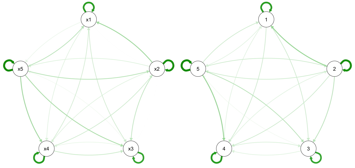
Finally, MCMSEM allows us to compare the two models in terms of fit, and in terms of fit to holdout data we generated previously.
MCMcompareloss(list(res.single.fac,res.network),test_data = simdata.holdout)
      mse_train_loss train_chisq   train_bic mse_test_loss  mse_diff mse_test_chisq mse_test_bic N_parameters
model1   0.4127585292 123827.5588 124079.7895    0.43718457        NA      65577.686    65816.054           20
model2   0.0003538882    106.1665    547.5703    0.01523786 0.4219467       2285.678     2702.822           35
So in the training data (data you used to fit the model) the loss of the network model is way lower than that of the factor model, so are the chi-square statistics, the BIC. In the test data we still have a lower loss for the network model, and a lower chi-square and BIC as well. The network model does have more parameters (complexity): 20 directed edges, 5 skewness parameters, 5 variances, and 5 kurtosis parameters. The added complexity outweighs the cost because the model does (way) better in new data.
This was the advertorial, there are practical theoretical and methodological nuances and limitations, but I bet you are motivated to learn about these now!
First simulate 20,000 independent subjects from a stationary bivariate VAR(1).
The rows of B_true are current outcomes and its columns are lagged predictors.
The two innovations are mutually independent, non-Gaussian, mean zero, and
variance one—the assumptions used by the fitted dynamic kernel.
library(MCMSEM)
library(lavaan)
set.seed(20260730)
n <- 20000L
B_true <- matrix(c(0.55, 0.16,
                  -0.12, 0.45), 2, 2, byrow = TRUE)
state <- matrix(0, n, 2)
panel <- array(NA_real_, dim = c(n, 2, 4))

innovation <- function(n) {
  cbind(
    rexp(n) - 1,
    (rchisq(n, df = 5) - 5) / sqrt(10)
  )
}

# Burn in for 200 transitions, then retain four consecutive waves.
for (tt in seq_len(204L)) {
  state <- state %*% t(B_true) + innovation(n)
  if (tt > 200L) panel[, , tt - 200L] <- state
}

sim_wide <- data.frame(
  X1 = panel[, 1, 1], Y1 = panel[, 2, 1],
  X2 = panel[, 1, 2], Y2 = panel[, 2, 2],
  X3 = panel[, 1, 3], Y3 = panel[, 2, 3],
  X4 = panel[, 1, 4], Y4 = panel[, 2, 4]
)
Fit an equality-constrained CLPM to all four waves. Because the data-generating process has no time-invariant trait component, a standard CLPM is the matched longitudinal estimator in this simulation.
sim_clpm <- "
  X2 ~ x_ar*X1 + y_to_x*Y1
  X3 ~ x_ar*X2 + y_to_x*Y2
  X4 ~ x_ar*X3 + y_to_x*Y3
  Y2 ~ y_ar*Y1 + x_to_y*X1
  Y3 ~ y_ar*Y2 + x_to_y*X2
  Y4 ~ y_ar*Y3 + x_to_y*X3
  X1 ~~ Y1
  X2 ~~ Y2
  X3 ~~ Y3
  X4 ~~ Y4
"
sim_clpm_fit <- sem(
  sim_clpm, data = sim_wide, estimator = "MLR", meanstructure = TRUE
)
Now discard waves 1–3 and fit the dynamic kernel to the final marginal cross-section only.
sim_final <- sim_wide[c("X4", "Y4")]
names(sim_final) <- c("X", "Y")
sim_ds <- MCMdatasummary(
  sim_final, scale_data = FALSE, prep_asymptotic_se = TRUE,
  use_skewness = TRUE, use_kurtosis = TRUE
)
sim_model <- MCMmodel(
  sim_ds, n_latent = 0, kernel = "dynamic",
  gaussian_residual = FALSE
)
sim_model <- MCMedit(sim_model, "B", c(1, 1), "x_ar")
sim_model <- MCMedit(sim_model, "B", c(1, 2), "y_to_x")
sim_model <- MCMedit(sim_model, "B", c(2, 1), "x_to_y")
sim_model <- MCMedit(sim_model, "B", c(2, 2), "y_ar")
sim_fit <- MCMfit(
  sim_model, sim_ds, compute_se = TRUE,
  optimizers = c("rprop", "lbfgs"), optim_iters = c(750, 40),
  learning_rate = c(0.01, 0.2),
  moment_weighting = "diagonal", se_correction = "robust",
  n_starts = 20, seed = 20260730, verbose = FALSE
)
The validated run recovered every transition closely:
Path (current <- lagged) |
Truth | CLPM estimate (SE) | Dynamic MCMSEM estimate (robust SE) |
|---|---|---|---|
| X <- X | 0.550 | 0.550 (0.003) | 0.555 (0.014) |
| X <- Y | 0.160 | 0.162 (0.004) | 0.147 (0.046) |
| Y <- X | -0.120 | -0.117 (0.003) | -0.111 (0.028) |
| Y <- Y | 0.450 | 0.446 (0.004) | 0.462 (0.014) |
The CLPM had robust CFI = 1.000, RMSEA = 0.000, and SRMR = 0.003. The dynamic solution had loss 0.000459, spectral radius 0.522, nominal df = 4, Jacobian rank 8/8, information condition number 1.81e4, and 20/20 admissible starts. This is the clean agreement expected when both estimators' assumptions match the data-generating process; it is not evidence that agreement is guaranteed with observational data.
Now simulate a second dataset from the same transition matrix, but add a time-invariant bivariate Gaussian random intercept to every wave. The dynamic innovations are centered, variance-one gamma variables with shapes 1 and 2.5. The random-intercept covariance is
      X    Y
X  0.50 0.20
Y  0.20 0.35
This data-generating process satisfies both fitted models: the RI-CLPM observes the stable Gaussian component across waves, while dynamic MCMSEM represents the same component as an additive Gaussian residual in the marginal cross-section. The larger sample reflects the power required to estimate a nearly saturated bivariate higher-moment decomposition.
set.seed(20260732)
n_ri <- 100000L
shape_x <- 1
shape_y <- 2.5
Psi_true <- matrix(c(0.50, 0.20,
                     0.20, 0.35), 2, 2, byrow = TRUE)
state_ri <- matrix(0, n_ri, 2)
panel_ri <- array(NA_real_, dim = c(n_ri, 2, 4))

innovation_ri <- function(n) {
  cbind(
    (rgamma(n, shape_x) - shape_x) / sqrt(shape_x),
    (rgamma(n, shape_y) - shape_y) / sqrt(shape_y)
  )
}

for (tt in seq_len(204L)) {
  state_ri <- state_ri %*% t(B_true) + innovation_ri(n_ri)
  if (tt > 200L) panel_ri[, , tt - 200L] <- state_ri
}

random_intercept <- matrix(rnorm(n_ri * 2L), n_ri, 2L) %*%
  chol(Psi_true)
for (wave in seq_len(4L)) {
  panel_ri[, , wave] <- panel_ri[, , wave] + random_intercept
}

sim_ri_wide <- data.frame(
  X1 = panel_ri[, 1, 1], Y1 = panel_ri[, 2, 1],
  X2 = panel_ri[, 1, 2], Y2 = panel_ri[, 2, 2],
  X3 = panel_ri[, 1, 3], Y3 = panel_ri[, 2, 3],
  X4 = panel_ri[, 1, 4], Y4 = panel_ri[, 2, 4]
)

# Reuse sim_clpm from the preceding example.
sim_confounded_clpm_fit <- sem(
  sim_clpm, data = sim_ri_wide, estimator = "MLR",
  meanstructure = TRUE
)
Fit the corresponding equality-constrained RI-CLPM:
sim_riclpm <- "
  RI_X =~ 1*X1 + 1*X2 + 1*X3 + 1*X4
  RI_Y =~ 1*Y1 + 1*Y2 + 1*Y3 + 1*Y4
  wX1 =~ 1*X1
  wX2 =~ 1*X2
  wX3 =~ 1*X3
  wX4 =~ 1*X4
  wY1 =~ 1*Y1
  wY2 =~ 1*Y2
  wY3 =~ 1*Y3
  wY4 =~ 1*Y4
  X1 ~~ 0*X1
  X2 ~~ 0*X2
  X3 ~~ 0*X3
  X4 ~~ 0*X4
  Y1 ~~ 0*Y1
  Y2 ~~ 0*Y2
  Y3 ~~ 0*Y3
  Y4 ~~ 0*Y4
  wX2 ~ x_ar*wX1 + y_to_x*wY1
  wX3 ~ x_ar*wX2 + y_to_x*wY2
  wX4 ~ x_ar*wX3 + y_to_x*wY3
  wY2 ~ y_ar*wY1 + x_to_y*wX1
  wY3 ~ y_ar*wY2 + x_to_y*wX2
  wY4 ~ y_ar*wY3 + x_to_y*wX3
  RI_X ~~ RI_Y
  wX1 ~~ wY1
  wX2 ~~ wY2
  wX3 ~~ wY3
  wX4 ~~ wY4
  RI_X ~~ 0*wX1 + 0*wY1
  RI_Y ~~ 0*wX1 + 0*wY1
"
sim_riclpm_fit <- sem(
  sim_riclpm, data = sim_ri_wide, estimator = "MLR",
  meanstructure = TRUE, fixed.x = FALSE
)
stopifnot(lavInspect(sim_riclpm_fit, "post.check"))
For MCMSEM, use only wave 4 and add the Gaussian residual. Because this is a calibration with known innovation families, constrain each innovation's skewness and excess kurtosis to the relationship implied by its freely estimated positive shape. The confounder remains fully Gaussian and its three covariance parameters remain free.
sim_ri_final <- sim_ri_wide[c("X4", "Y4")]
names(sim_ri_final) <- c("X", "Y")
sim_ri_ds <- MCMdatasummary(
  sim_ri_final, scale_data = FALSE, prep_asymptotic_se = TRUE,
  use_skewness = TRUE, use_kurtosis = TRUE
)
sim_gaussian_model <- MCMmodel(
  sim_ri_ds, n_latent = 0, kernel = "dynamic",
  residual_family = "gaussian"
)
sim_gaussian_model <- MCMedit(
  sim_gaussian_model, "B", c(1, 1), "x_ar"
)
sim_gaussian_model <- MCMedit(
  sim_gaussian_model, "B", c(1, 2), "y_to_x"
)
sim_gaussian_model <- MCMedit(
  sim_gaussian_model, "B", c(2, 1), "x_to_y"
)
sim_gaussian_model <- MCMedit(
  sim_gaussian_model, "B", c(2, 2), "y_ar"
)
sim_gaussian_model <- MCMparameter(
  sim_gaussian_model, "shape_X", "free",
  start = shape_x, transform = "positive"
)
sim_gaussian_model <- MCMparameter(
  sim_gaussian_model, "shape_Y", "free",
  start = shape_y, transform = "positive"
)
sim_gaussian_model <- MCMparameter(
  sim_gaussian_model, "sign_X", "fixed", value = 1
)
sim_gaussian_model <- MCMparameter(
  sim_gaussian_model, "sign_Y", "fixed", value = 1
)
sim_gaussian_model <- MCMparameter(
  sim_gaussian_model, "tau_X", "derived",
  expression = ~ sign_X * 2 / sqrt(shape_X)
)
sim_gaussian_model <- MCMparameter(
  sim_gaussian_model, "kappa_X", "derived",
  expression = ~ 6 / shape_X
)
sim_gaussian_model <- MCMparameter(
  sim_gaussian_model, "tau_Y", "derived",
  expression = ~ sign_Y * 2 / sqrt(shape_Y)
)
sim_gaussian_model <- MCMparameter(
  sim_gaussian_model, "kappa_Y", "derived",
  expression = ~ 6 / shape_Y
)

# For this calibration only, initialize one of the ten starts at the known
# generating values. The other nine starts are randomized as usual.
calibration_starts <- c(
  x_ar = 0.55, y_to_x = 0.16, x_to_y = -0.12, y_ar = 0.45,
  shape_X = 1, shape_Y = 2.5,
  log_sd_G_X = -0.346574,
  chol_G_Y_X = 0.282843,
  log_sd_G_Y = -0.654667
)
for (name in names(calibration_starts)) {
  sim_gaussian_model <- MCMedit(
    sim_gaussian_model, "start", name, calibration_starts[[name]]
  )
}

sim_gaussian_fit <- MCMfit(
  sim_gaussian_model, sim_ri_ds, compute_se = TRUE,
  optimizers = c("rprop", "lbfgs"), optim_iters = c(700, 60),
  learning_rate = c(0.01, 0.05),
  moment_weighting = "diagonal", se_correction = "robust",
  n_starts = 10, seed = 20260732, verbose = FALSE
)
The ordinary CLPM mixes the stable intercept into the observed-score paths. The RI-CLPM and Gaussian-residual MCMSEM instead recover the generating within-person transition within sampling uncertainty:
Path (current <- lagged) |
Truth | CLPM estimate (SE) | RI-CLPM estimate (SE) | Gaussian MCMSEM estimate (robust SE) |
|---|---|---|---|---|
| X <- X | 0.550 | 0.646 (0.001) | 0.548 (0.003) | 0.530 (0.023) |
| X <- Y | 0.160 | 0.172 (0.001) | 0.165 (0.003) | 0.207 (0.040) |
| Y <- X | -0.120 | -0.046 (0.001) | -0.118 (0.003) | -0.101 (0.016) |
| Y <- Y | 0.450 | 0.576 (0.002) | 0.452 (0.003) | 0.476 (0.028) |
All four generating paths fall inside the MCMSEM robust 95% intervals. The estimated Gaussian residual covariance was
      X     Y
X 0.485 0.132
Y 0.132 0.331
versus the generating covariance shown above. MCMSEM had loss 0.000222,
spectral radius 0.523, nominal df = 3, Jacobian rank 9/9, and information
condition number
This example uses the U.S. Census Bureau's public-use 2014 Survey of Income and Program Participation (SIPP) panel. Its four waves cover the 2013--2016 reference years. The original Census files are hundreds of megabytes and are not stored in this repository. Instead, the package includes a 437 KB derived analysis matrix and its full provenance.
The matrix contains only four waves of transformed log earnings and usual weekly hours: eight columns, no identifiers, demographics, survey weights, or source variables. The derivation selected December in each wave, retained a working-age baseline cohort, and treated non-positive earnings or hours as unavailable. The analysis is consequently an unweighted methodological illustration among people with positive earnings and hours, not a population-representative labor estimate. Variable definitions and the public-use files are available from the Census wave pages and data dictionaries.
Load the exact matrix used below:
library(MCMSEM)
library(lavaan)

sipp_file <- system.file(
  "extdata", "sipp_2014_panel.csv.gz", package = "MCMSEM"
)
if (!nzchar(sipp_file)) {
  # When running directly from a source checkout.
  sipp_file <- "inst/extdata/sipp_2014_panel.csv.gz"
}
sipp <- read.csv(sipp_file, na.strings = c("", "NA"))
stopifnot(
  identical(
    names(sipp),
    c(
      "Earnings1", "Hours1", "Earnings2", "Hours2",
      "Earnings3", "Hours3", "Earnings4", "Hours4"
    )
  )
)
Log earnings and hours were each centered using wave-1 complete cases and
rescaled as 2 * (value - wave1_mean) / wave1_sd. The same affine
transformation was used at every wave and in every model. It gives both
variables variance four in wave 1, comfortably above the dynamic kernel's fixed
unit innovation variance. Thus the reported unstandardized paths share common
measurement units and are approximately standardized; scale differences do not
explain differences between methods.
Dynamic MCMSEM assumes a stationary marginal distribution, so in the population any wave could be used. We use wave 1 because it has the largest jointly observed sample. The empirical moments are similar but not identical, so stationarity remains an approximation rather than something established by choosing the largest wave:
| Wave | Reference year | Complete N | Earnings mean | Hours mean | Earnings variance | Hours variance | Covariance |
|---|---|---|---|---|---|---|---|
| 1 | 2013 | 22,049 | 0.000 | 0.000 | 4.000 | 4.000 | 2.031 |
| 2 | 2014 | 15,787 | 0.036 | -0.034 | 4.192 | 4.170 | 2.179 |
| 3 | 2015 | 12,190 | 0.184 | 0.055 | 4.012 | 4.205 | 2.087 |
| 4 | 2016 | 10,446 | 0.268 | 0.033 | 4.057 | 4.156 | 2.166 |
Fit three complementary models from the outset. The CLPM describes observed-score dynamics, the RI-CLPM separates stable between-person differences from within-person change, and dynamic MCMSEM uses a Gaussian residual to represent a stable marginal component. The four transition paths are constrained equal across the three annual panel transitions. MLR and FIML retain incomplete panel rows and provide non-normality-robust inference.
clpm_syntax <- "
  Earnings2 ~ earnings_ar*Earnings1 + hours_to_earnings*Hours1
  Earnings3 ~ earnings_ar*Earnings2 + hours_to_earnings*Hours2
  Earnings4 ~ earnings_ar*Earnings3 + hours_to_earnings*Hours3

  Hours2 ~ hours_ar*Hours1 + earnings_to_hours*Earnings1
  Hours3 ~ hours_ar*Hours2 + earnings_to_hours*Earnings2
  Hours4 ~ hours_ar*Hours3 + earnings_to_hours*Earnings3

  Earnings1 ~~ Hours1
  Earnings2 ~~ Hours2
  Earnings3 ~~ Hours3
  Earnings4 ~~ Hours4
"
clpm_fit <- sem(
  clpm_syntax, data = sipp,
  estimator = "MLR", missing = "fiml", meanstructure = TRUE
)
Prepare the largest complete cross-section for both MCMSEM residual-family fits used below:
complete_n <- vapply(seq_len(4L), function(wave) {
  sum(complete.cases(sipp[paste0(c("Earnings", "Hours"), wave)]))
}, integer(1))
mcm_wave <- which.max(complete_n)
mcm_values <- na.omit(
  sipp[paste0(c("Earnings", "Hours"), mcm_wave)]
)
names(mcm_values) <- c("Earnings", "Hours")

dynamic_data <- MCMdatasummary(
  mcm_values,
  scale_data = FALSE,
  prep_asymptotic_se = TRUE,
  use_skewness = TRUE,
  use_kurtosis = TRUE
)

make_dynamic_model <- function(residual_family) {
  model <- MCMmodel(
    dynamic_data,
    n_latent = 0,
    kernel = "dynamic",
    residual_family = residual_family
  )
  model <- MCMedit(model, "B", c(1, 1), "Earnings_AR")
  model <- MCMedit(
    model, "B", c(1, 2), "Hours_lag_to_Earnings"
  )
  model <- MCMedit(
    model, "B", c(2, 1), "Earnings_lag_to_Hours"
  )
  MCMedit(model, "B", c(2, 2), "Hours_AR")
}
A CLPM mixes stable between-person differences with within-person change. The RI-CLPM below separates two correlated random intercepts from within-person deviations and estimates the transition matrix among those deviations.
riclpm_syntax <- "
  RI_Earnings =~ 1*Earnings1 + 1*Earnings2 + 1*Earnings3 + 1*Earnings4
  RI_Hours =~ 1*Hours1 + 1*Hours2 + 1*Hours3 + 1*Hours4

  wE1 =~ 1*Earnings1
  wE2 =~ 1*Earnings2
  wE3 =~ 1*Earnings3
  wE4 =~ 1*Earnings4
  wH1 =~ 1*Hours1
  wH2 =~ 1*Hours2
  wH3 =~ 1*Hours3
  wH4 =~ 1*Hours4

  Earnings1 ~~ 0*Earnings1
  Earnings2 ~~ 0*Earnings2
  Earnings3 ~~ 0*Earnings3
  Earnings4 ~~ 0*Earnings4
  Hours1 ~~ 0*Hours1
  Hours2 ~~ 0*Hours2
  Hours3 ~~ 0*Hours3
  Hours4 ~~ 0*Hours4

  wE2 ~ earnings_ar*wE1 + hours_to_earnings*wH1
  wE3 ~ earnings_ar*wE2 + hours_to_earnings*wH2
  wE4 ~ earnings_ar*wE3 + hours_to_earnings*wH3
  wH2 ~ hours_ar*wH1 + earnings_to_hours*wE1
  wH3 ~ hours_ar*wH2 + earnings_to_hours*wE2
  wH4 ~ hours_ar*wH3 + earnings_to_hours*wE3

  RI_Earnings ~~ RI_Hours
  wE1 ~~ wH1
  wE2 ~~ wH2
  wE3 ~~ wH3
  wE4 ~~ wH4
  RI_Earnings ~~ 0*wE1 + 0*wH1
  RI_Hours ~~ 0*wE1 + 0*wH1
"
riclpm_fit <- sem(
  riclpm_syntax, data = sipp,
  estimator = "MLR", missing = "fiml",
  meanstructure = TRUE, fixed.x = FALSE
)
stopifnot(lavInspect(riclpm_fit, "post.check"))
In dynamic MCMSEM, residual_family = "gaussian" adds an unrestricted
Gaussian covariance that is not propagated through the transition matrix. It
is conceptually analogous to a joint distribution of stable between-person
differences: it can absorb variance and covariance that should not be assigned
to the dynamic innovations. Unlike the RI-CLPM, however, a one-wave MCMSEM fit
does not observe that the component persists over time; stability is a
distributional interpretation.
gaussian_model <- make_dynamic_model("gaussian")
gaussian_fit <- MCMfit(
  gaussian_model,
  dynamic_data,
  compute_se = TRUE,
  optimizers = c("rprop", "lbfgs"),
  optim_iters = c(1400, 80),
  learning_rate = c(0.01, 0.005),
  moment_weighting = "diagonal",
  se_correction = "robust",
  n_starts = 20,
  seed = 20260731,
  verbose = FALSE
)
gaussian_fit$Psi_G
Path (current <- lagged) |
CLPM estimate (robust SE) | RI-CLPM estimate (robust SE) | Gaussian MCMSEM estimate (robust SE) |
|---|---|---|---|
| Earnings <- earnings | 0.628 (0.011) | 0.105 (0.024) | 0.627 (0.091) |
| Earnings <- hours | 0.063 (0.008) | 0.051 (0.012) | 0.127 (0.104) |
| Hours <- earnings | 0.124 (0.007) | 0.009 (0.015) | 0.465 (0.116) |
| Hours <- hours | 0.476 (0.009) | 0.165 (0.017) | 0.591 (0.163) |
The CLPM used all 24,505 contributing panel rows; scaled CFI, TLI, RMSEA, and SRMR were 0.905, 0.867, 0.052, and 0.086. The RI-CLPM passed lavaan's post-estimation check and fit the longitudinal covariance structure closely: scaled CFI = 0.998, TLI = 0.996, RMSEA = 0.009, and SRMR = 0.012. The MCMSEM Gaussian residual covariance was
          Earnings  Hours
Earnings     1.842  0.450
Hours        0.450  0.421
which implies a residual correlation of 0.511. Its loss was 0.1004, spectral
radius 0.852, nominal df = 1, and Jacobian rank 11/11. The information
condition number was
A Gaussian residual affects covariance and Gaussian fourth-moment pairings but
has no third or fourth cumulants. If the stable source is skewed, assigning all
higher cumulants to the dynamic innovations may distort the transition matrix.
The common-gamma family adds one centered variance-one gamma factor U with
signed loadings lambda:
Its positive shape alpha determines skewness alpha approaches a rank-one Gaussian
factor. Loadings remain signed, so odd cumulants retain their direction.
The direct API is:
gamma_model <- make_dynamic_model("common_gamma")The most flexible currently supported specification leaves the diagonal third and fourth innovation cumulants free. It is therefore a common-gamma residual or confounder combined with innovation skewness and kurtosis that are estimated independently rather than tied to a named distribution. "Unspecified" here means through the fitted fourth order: innovations still have fixed unit variances, are mutually independent, and have diagonal third- and fourth-order cumulants. This is a reasonable specification when a shared gamma-shaped source is plausible but no parametric innovation family can be defended. However, the bivariate model estimates 11 parameters from 12 moments, leaving only one nominal overidentifying degree of freedom and allowing competing, ill-conditioned decompositions.
As a more restrictive sensitivity analysis, we also imposed a scientifically explicit signed-gamma relationship on each innovation. Earnings innovations were allowed negative skew and hours innovations positive skew, while their two shapes remained free. This reduces the free parameter count and leaves three nominal df. For example:
gamma_model <- MCMparameter(
  gamma_model, "shape_Earnings", "free",
  start = 0.114, transform = "positive"
)
gamma_model <- MCMparameter(
  gamma_model, "shape_Hours", "free",
  start = 0.295, transform = "positive"
)
gamma_model <- MCMparameter(
  gamma_model, "sign_Earnings", "fixed", value = -1
)
gamma_model <- MCMparameter(
  gamma_model, "sign_Hours", "fixed", value = 1
)
gamma_model <- MCMparameter(
  gamma_model, "tau_Earnings", "derived",
  expression = ~ sign_Earnings * 2 / sqrt(shape_Earnings)
)
gamma_model <- MCMparameter(
  gamma_model, "kappa_Earnings", "derived",
  expression = ~ 6 / shape_Earnings
)
gamma_model <- MCMparameter(
  gamma_model, "tau_Hours", "derived",
  expression = ~ sign_Hours * 2 / sqrt(shape_Hours)
)
gamma_model <- MCMparameter(
  gamma_model, "kappa_Hours", "derived",
  expression = ~ 6 / shape_Hours
)

# A direct multistart fit. The validation script below uses a broader explicit
# grid over confounder shapes and loading orientations.
gamma_fit <- MCMfit(
  gamma_model,
  dynamic_data,
  compute_se = TRUE,
  optimizers = c("rprop", "lbfgs"),
  optim_iters = c(1200, 100),
  learning_rate = c(0.01, 0.005),
  moment_weighting = "diagonal",
  se_correction = "robust",
  n_starts = 30,
  seed = 20260902,
  verbose = FALSE
)
gamma_fit$dynamic$common_gamma
The validation script searches both loading orientations and several starting shapes before computing robust SEs for both innovation specifications.
For convenience, the table repeats all three preceding fits alongside the two common-gamma results:
Path (current <- lagged) |
CLPM (robust SE) | RI-CLPM (robust SE) | Gaussian MCMSEM (robust SE) | Common gamma + signed-gamma innovations (robust SE) | Common gamma + free innovation cumulants (robust SE) |
|---|---|---|---|---|---|
| Earnings <- earnings | 0.628 (0.011) | 0.105 (0.024) | 0.627 (0.091) | 0.676 (0.032) | 0.494 (0.058) |
| Earnings <- hours | 0.063 (0.008) | 0.051 (0.012) | 0.127 (0.104) | 0.075 (0.052) | 0.284 (0.047) |
| Hours <- earnings | 0.124 (0.007) | 0.009 (0.015) | 0.465 (0.116) | 0.422 (0.030) | 0.459 (0.046) |
| Hours <- hours | 0.476 (0.009) | 0.165 (0.017) | 0.591 (0.163) | 0.651 (0.036) | 0.579 (0.037) |
The common-factor loadings were -1.347 (SE 0.108) for earnings and -0.360
(SE 0.235) for hours. Their product gives a positive rank-one covariance. The
estimated gamma shape was 153.8 (SE 398.2), implying skewness 0.161
(SE 0.209) and excess kurtosis 0.039 (SE 0.101). The loss was 0.1090 and the
information condition number was
This fit does not provide reliable evidence that the confounder is non-Gaussian: the point estimate is close to the Gaussian limit, its distributional SEs are large, and the overall decomposition is extremely ill-conditioned. That conclusion is conditional on the signed-gamma innovation constraints; it is not a general test that every possible confounder is Gaussian.
The extended free-innovation grid found a basin with loss 0.000231, shape 0.486
(SE 0.086), and loadings 1.214 (SE 0.039) for earnings and -0.063 (SE 0.037)
for hours. Its information condition was
The freely estimated innovation third and fourth cumulants were -10.943 (SE 1.870) and 73.207 (SE 9.859) for earnings, and 4.233 (SE 0.463) and 24.045 (SE 1.887) for hours. Because innovation variances are fixed to one, these are also the innovations' skewness and excess kurtosis. Thus, this basin combines strongly non-Gaussian innovations with the gamma residual component; it does not attribute all higher-moment structure to the residual.
Several positive-loading-orientation starts converged to nearby versions of this basin, whereas the negative-orientation fits had appreciably higher loss. That multistart stability supports the existence of the basin but does not remove the weak-identification warning implied by one df and the large information condition.
Although the model permits a shared gamma confounder, this fitted gamma component is almost entirely specific to earnings because the hours loading is small and imprecise. It is evidence for an earnings-specific strongly non-Gaussian residual under this specification, not convincing evidence for a shared earnings-hours confounder. Run the unrestricted-innovation sensitivity analysis with
Rscript inst/validation/longitudinal_clpm_example.R --unrestricted-gammaThe constrained and unrestricted results together show that the data do not support a specification-invariant conclusion about confounder shape.
These comparisons should be read as triangulation rather than as competing software implementations of one regression:
- The CLPM identifies observed-score paths from repeated transitions. Dynamic MCMSEM reconstructs a stationary transition from one marginal distribution and higher cumulants.
- The RI-CLPM and residual-adjusted MCMSEM both attempt a within-versus-between decomposition. The RI-CLPM observes stable components across waves; MCMSEM infers a residual distribution under stronger assumptions.
- A residual family can improve the scientific match while weakening identification. Compare Jacobian rank, information condition, nominal df, spectral radius, multistart behavior, and robust SEs—not only training loss.
- The controlled simulations demonstrate that CLPM and plain MCMSEM can agree without a stable component, and that RI-CLPM and Gaussian-residual MCMSEM can agree when a Gaussian stable component is present. Real-data estimates do not have to converge: disagreement can reflect different estimands, nonstationarity, weak distributional identification, or model misspecification rather than a scaling error.
The complete executable analysis, including the simulation, all multistart
settings, wave diagnostics, and machine-readable output, is in
inst/validation/longitudinal_clpm_example.R;
a compact record of the validated results is in
inst/validation/longitudinal_clpm_example.md.
For a more detailed description of the various functions used, see our wiki pages.
If you would like to contribute to MCMSEM, please do so via the dev-torch branch.