February 2018 by Irene Mavilia (ISAC-CNR, i.mavilia@isac.cnr.it)
A Python tool, composed of packages that are collections of modules, is designed to identify significant recurrent structures (clusters) in a dataset, which are also analysed performing diagnostics and computing metrics. The starting point is time filtering and reduction to low dimensional Principal Components (PC) space. Then the k-means algorithm seeks to partition all states into k clusters minimising the intra-cluster distance and maximising the distance among the cluster centroids. Diagnostics regard the spatial pattern and the index of occurrence frequencies of the extracted structures, while metrics refer to pattern correlation, mean squared error, phase error (measures of the differences between maps) and significance of cluster partition with respect to a reference dataset (e.g. observations). All the resulting output can be saved in ASCII and netCDF formats as well as plotted in figures.
arrange_inputdata.sh Before the weather regime analysis, data should be remap r144x73 and the period of interest should be selected. arrange_inputdata.sh allows to do that with cdo.
inputCLUS_tool.sh Set the information required by the WRTOOL: this shell wrapper collects the following set of parameters, required by the WRTOOL. Write only letters or numbers, no symbols or punctuation marks! If you do not want to set a certain parameter write 'no' (e.g. enstoselect=no)
-------------------------------about paths------------------------------------------
- WRTOOL_PATH: WRTOOL directory
- OUTPUT_PATH: output folder
- INPUT_PATH: directory that contains the input data
- List of input files: filenames[0]='???.nc' to filename[n]='???.nc'
-------------------------------about data-------------------------------------------
- varname: variable name as in the input file (zg,...)
- level: level to select if variable contains more levels (500,...)
- freq: data frequency (day, mon, year,...)
- filterwnd: running mean filter time window (5,...)
- varunits: variable units (m,...)
- model: model name (ECEARTH31, NCEPNCAR, ERAInterim,...)
- kind: kind of input data (obs: observations, base: baseline, stoc: stochastic physics,...)
- res: resolution (144x73, T255,...)
- numens: total number of ensemble members
- enstoselect: single ensemble member to analyse (starting from 0!) If you have only one realization set numens=1 and enstoselect=no If you have more than one ensemble member: if you set enstoselect=3, as an example, only member 3 will be analysed; otherwise with enstoselect=no, all the numens ensemble member fields are concatenated in time before the analysis and the clusters are computed on the resulting field.
- season: season to be selected (DJF, DJFM, NDJFM, JJA)
- area: regional average (EAT: Euro-Atlantic, PNA: Pacific North America, NH: Northern Hemisphere)
- syr: starting year
- eyr: end year
---------------------about cluster analysis------------------------------------------
- numclus: number of clusters Either set perc or numpcs (write '...=no' to the parameter you do not want to set):
- perc: percentage of explained variance (cluster analysis is applied on a number of PCs such as they explain perc of total variance)
- numpcs: number of PCs (cluster analysis is applied on numpcs Principal Components)
- nameREF: reference name files required by clusters_comparson.py
CLUS_tool.sh At the beginning, this script activates the cdms2 environment, which contains all the needed modules, and deactivates it at the end.
precompute.py It prepares data for the analysis: If it does not exist, it creates the output directory It reads the netCDF file of (lat, lon, lev, variable) for one or more ensemble members (if there are more members, they should be the only files present in INPUT_PATH). It can select one level, a season, it can filter by running mean and compute anomalies by removing the time-mean for each time (e.g. day), then it can select an area. It saves the resulting netCDF field of anomalies (lat, lon, anomalies).
compute.py It performs the analysis: It loads the netCDF field of anomalies saved by precompute.py, if enstoselect is set to a value, it selected only that member for the analysis, otherwise all ensemble members are concatenated one after the other prior to the analysis. It computes empirical orthogonal functions EOFs and principal components PCs of the loaded field of anomalies weighted by the square root of the cosine of latitude. It plots the first EOF (multiplied by the square-root of their eigenvalues) and the first PC (divided by the square-root of their eigenvalues) and it saves the first numpcs EOFs and PCs (scaled and unscaled), jointly with the the fractional variance represented by each EOF mode.
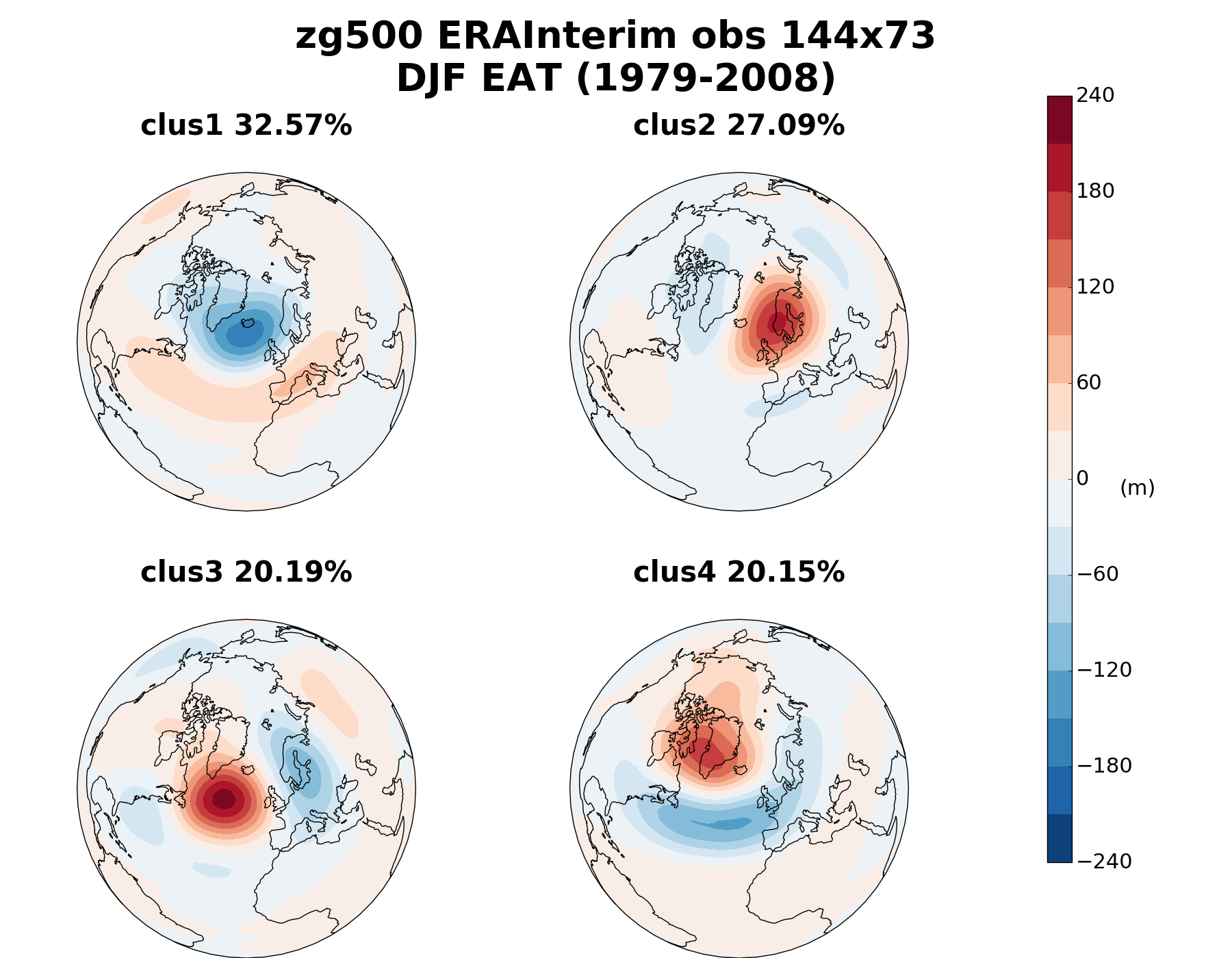
clustering.py It seeks numclus clusters via k-means algorithm for a subset of numpcs unscaled PCs: It saves the cluster index (each time is labelled with an integer from 0 to numclus) and the cluster centroids coordinates and the optimal variance ratio, which is the ratio between the variance among the centroid clusters and the intra-cluster variance. It sorts the clusters by decreasing frequency of occurrence. It plots and save the cluster spatial patterns (the average of the original field of anomalies during times belonging to that cluster).
clusters_comparison.py It finds the best possible match between two sets of cluster partitions: It computes and saves the projections of the simulated cluster patterns and the reference cluster patterns onto the same reference EOF patterns, obtaining vectors in the PC space (numpcs dimensions). It compares the two cluster partitions computing the total squared error, the phase error, the pattern correlation and the combination that minimizes the mean total squared error, which can be used to order the simulated clusters as the reference. It sorts the clusters as the reference.
clusters_sig.py It computes an saves the significance of the cluster partition, starting from PCs and varopt.
clusters_plots.py It produces and saves plots of weather regimes' patterns.
Only the first time before using it on a different system you need:
- To create the environment cdms2 from the environment.yml file:
conda env create -f environment.yml
conda list
- To compile ctool.so and ctp.so modules in cluster_fortran folder:
f2py --fcompiler=gfortran --f90flags="-fopenmp" -lgomp -c -m ctp cluster_toolkit_parallel.f90 only: clus_sig_p
f2py --fcompiler=gfortran -c -m ctool cluster_toolkit.f90 only: clus_opt adran1 gausts tsstat
- To run the tool you need to modify the inputCLUS_tool.sh with correct paths and parameters, and then launch CLUS_tool.sh First you need to run the tool for the reference data (like observations), in order to have the output needed to compare model data to observations. Then you can run the tool for your model data.
Dawson, Andrew, and T. N. Palmer. "Simulating weather regimes: Impact of model resolution and stochastic parameterization." Climate Dynamics 44, no. 7-8 (2015): 2177-2193.
Straus, David M., Susanna Corti, and Franco Molteni. "Circulation regimes: Chaotic variability versus SST-forced predictability." Journal of climate 20, no. 10 (2007): 2251-2272.